


Introduction
The Copenhagen meeting on climate change reflected the conflicting aims of those countries that industrialised at an early stage and are mainly responsible for current high greenhouse gas levels, those that are now in the course of rapid industrialisation, and those that remain undeveloped. The lack of agreement on effective measures may also reflect uncertainty that the warming detected over the last few decades is, in fact, attributable to human activity and uncertainty that climate will continue to get warmer and sea-level to rise if the input of greenhouse gases (GHG –see Glossary–) to the atmosphere is not greatly reduced.
Most climatologists are convinced that global temperatures have increased since the beginning of the industrial revolution and that the increase is mainly attributable to increased concentrations of greenhouse gases of anthropogenic origin in the atmosphere, especially carbon dioxide, and that if nothing is done to restrict future inputs global temperatures will continue to increase with potentially disastrous consequences, including water shortages in many areas, greater weather extremes and coastal flooding.
Many non-climatologists are unconvinced that mankind is capable of changing the climate. They are inclined to believe that any warming that may have taken place in recent years is no more than a fluctuation of the kind that has happened many times in the past and is unlikely to persist for any great length of time into the future. They point to the views of many scientists and publicists who disagree with climatologists on the influence of greenhouse gases and who point to what they consider to be more important natural influences on climate, especially volcanic eruptions and variations in solar radiation. Some believe that there have been changes in global temperature in historic times exceeding any that have occurred since the beginning of the industrial revolution. They may even argue that the beneficial fertilising effects of carbon dioxide outweigh any detrimental effects of the potential warming it may cause. Because of their doubts they see measures to restrict the burning of fossil fuels as being only harmful, liable to restrain future economic growth and likely to cause greater poverty in the developing world.
This Working Paper reviews the main reasons why definite and conclusive evidence in the field of climate change is almost an impossibility. It analyses the main elements that explain natural climatic change and reflects on the high level of uncertainty in the system, which in many ways is inherent to the system itself, and presents the latest evidence.
The following section presents in a stylised fashion the key features of uncertainty and how it relates to climate change. Then, an analysis of how GHG have been measured is followed by a discussion of the different GHG, natural and human-induced events that have a significant bearing on climate change. The Working Paper concludes with an overview of past, present and future climate change and with a summary of the main ideas discussed throughout the text.
Key Sources of Uncertainty in Climate Change
The record of global climate change in the historic past is uncertain because reliable instrumental records are limited to the last century or two, and to only a small proportion of the globe. However, it seems likely that global temperatures varied more over the last century than over the preceding millennium.
Predictions of how much temperature will rise in the 21st century are uncertain because the response of the climate to changing greenhouse gas concentrations, the rate of ocean heat uptake and the effects of cloud cover and aerosols are all poorly quantified.
Future natural influences on climate, such as solar output and volcanic eruptions, are at present unpredictable, and so are future levels of methane in the atmosphere.
Future sea-level changes are uncertain because of the difficulty of predicting precipitation on Antarctica and of determining the stability or otherwise of the West Antarctic and Greenland ice sheets.
Anthropogenic influences, such as world population growth, the nature of technological and economic development, the effects of land-use changes and the success or otherwise of efforts to restrain the growth of greenhouse gas concentrations in the atmosphere are uncertain.
Regional climate changes are even more difficult to predict than global changes. There is no doubt they will involve greater departures from current long-term means than will global changes.
Figure 1. Main water-related uncertainties in climate change applied to Spain
| How will the mean annual precipitation and inter-annual precipitation variability change for Spain? |
| How will the geographic distribution of precipitation change across Spain? |
| How will seasonal distribution of precipitation change? |
| How will the precipitation distribution function change at various temporal scales? |
| What will the consequences be of the variability of extreme precipitation events above a certain threshold for different time intervals? |
| Will droughts be more frequent and/or more intense? |
| How will the relationship of precipitation as rain or snow vary in mountain areas? |
| How will the evapo-transpiration and evaporation rates vary? |
Source: Mestre (2008).
The Discovery of Carbon-dioxide Warming
It was widely appreciated early in the 20th century that temperatures in many parts of the world had been rising for several decades. C.E.P. Brooks pointed out in Climate Through the Ages (1926), that over the preceding 100 years glaciers had been in rapid retreat in both hemispheres. Subsequently, temperature records for the 1920s and 1930s pointed to an accentuation of the warming trend.
Figure 2. Svante Arrhenius, Nobel Prize for Chemistry 1903
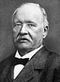
Guy Callendar (1938), an engineer with wide interests, was one of a small group of scientists who suspected that the warming might be associated with increasing concentrations of carbon dioxide in the atmosphere. Forty years earlier Svante Arrhenius had suspected that the cause of the Ice Ages might lie in lower concentrations of carbon dioxide in the atmosphere. His colleague, Högbom, pointed out that coal burning was adding carbon dioxide to the atmosphere at a significant rate and Arrhenius calculated that, if atmospheric concentrations were to double, global temperatures would rise by 5º-6oC. To many it seemed unlikely that such a relatively rare constituent of the atmosphere as carbon dioxide, only a few parts in 10,000, could have such an effect on the world’s climate and, in any case, at the rates of coal consumption then current, a doubling of carbon dioxide concentration lay centuries ahead. Anyway, climate had always been fluctuating and would, no doubt they thought, continue to do so.
There were other more serious objections to CO2 warming. It seemed likely that the oceans would absorb any additional carbon dioxide. Furthermore, it was widely accepted that water vapour, known to be a much more effective interceptor of infrared radiation than CO2, must block the bands of the spectrum where CO2 could be effective. However, in 1931 Hulburt showed that the structure of the absorption bands was much more elaborate than had been envisaged and that the spacing of the bands might allow a doubling of the CO2 concentration in the atmosphere, enough to produce a rise in temperature, it was thought, of 4oC. Callendar calculated that carbon dioxide concentrations had increased by 10% over the preceding century, enough to explain the warming that had taken place in that time.
With the outbreak of the Second World War in 1939 more immediate matters diverted attention from such considerations. Afterwards, Callendar returned to the topic. He produced evidence of temperature continuing to rise in many parts of the world and rejected the possibilities that the warming might be due to increasing levels of solar radiation or changing levels of dust in the atmosphere. Although he neglected to consider the part played by convection in atmospheric energy transport (ie, the fact that moist convection causes the release of latent heat and is important to the Earth’s energy budget), he recognised that the accompanying changes in cloud cover presented some difficulties in assessing the effect of carbon dioxide on temperature.
There was still the possibility that the oceans would absorb most of the additional carbon dioxide. Callendar thought this was unlikely to be the case and in 1957 Revelle and Suess showed he was right. The rate at which sea-water can take up carbon dioxide is limited and unable to cope with the rapidly increasing amounts being supplied to the atmosphere by the burning of fossil fuels. The explanation lies in the fact that most of the gas entering the surface water promptly evaporates back into the air before it is confined to greater depths by the slow circulation of the ocean. Revelle warned that the consequent effect on climate of increasing carbon dioxide concentrations might be radical and about the same time, Budyko, a prominent Russian climatologist, warned of the possibility of drastic global warming within the next century.
In the 1950s and 1960s, there was increased funding in the US for atmospheric and oceanographic research, especially associated with the threat from Soviet Russia. The International Geophysical Year of 1957-8 saw the application in the Earth sciences of new knowledge and new techniques especially involving radioactive isotopes. These stimulated revolutions in the Earth sciences and the biological sciences, with the development of various new methods for measuring and dating events in climate history.
In the 1960s global temperatures ceased to rise. It became apparent that permanent snow cover was increasing, on Baffin Island for instance and elsewhere in the Arctic, and glaciers in many parts of the world began to advance. Radiocarbon dating confirmed that the present interglacial period had already lasted about 10,000 years and some climatologists began to wonder if the cooling might point to the beginnings of a new glacial period.
At about this time Keeling’s measurements of carbon dioxide in the atmosphere, which he had started taking on Mauna Loa in 1958, were beginning to show that concentrations were increasing year by year, with regular seasonal fluctuations that could be attributed to the greater uptake by vegetation in Northern Hemisphere summers than in Southern Hemisphere summers. Rachel Carson’s Silent Spring, appearing in 1962, drew widespread public attention to man’s impact on nature, particularly the hazards associated with the pesticide DDT.
Until this time, both the long-term history of climate and the future prospect had been the concerns of a relatively few specialists, some of them historians and geographers, others scattered through the ecological and Earth sciences. Prominent amongst them was Hubert Lamb who, after a long career leading climate-variation research in the British Meteorological Office, established the Climatic Research Unit (CRU) at the University of East Anglia in 1971 and was appointed its first head. His book, Climate: Present, Past and Future, appeared the following year and was followed in 1982 by Climate, History and the Modern World.
In 1978 the CRU began to assemble temperature data sets for the world’s land areas, plotting them in 5o latitude/longitude boxes and deriving from the result a measure of terrestrial temperature change. In 1986, in cooperation with the Hadley Centre of the British Met Office, the procedure was extended to the marine sector. This work provided the basis for the first truly global temperature record. In addition, precipitation and other data bases were assembled and efforts were made to place the instrumental data in a longer time context, making use of tree ring records.
All this involveda great deal of painstaking work by a relatively small staff. It entailed corresponding with overseas meteorological services, begging for long weather records, requesting permissions to publish, attempting to take into account changes in the location and exposure of recording stations, and interpolating missing values for many locations. Subsequently, the CRU supplied several researchers in the UK and overseas with climatic data for their ecological and other studies. It is not very surprising that some of the long-serving members of the staff felt they had a proprietary interest in the raw material. Quite recently, in February 2010, the British Meteorological Office, following on from the pioneer work of the University of East Anglia, proposed a programme to deliver a new global temperature data set providing information on changing extremes and regional variability. It is intended that the new data set should be fully peer reviewed and open to scrutiny.
In the course of the 1970s the general public became increasingly aware of threats to the environment resulting from modern technical progress and industrial activity. The discovery in 1984 of the ozone hole over Antarctica by Farman et al (1985), British Antarctic Survey scientists, demonstrated that trace gases could have a dangerous influence on the atmosphere. Then, in the late 1980s, the work at the Climatic Research Unit showed that global temperatures were beginning to rise and the question as to whether the warming was natural or man-made attracted increasing attention.
In 1989 the World Meteorological Organisation (WMO) and the United Nations Environment Programme set up the International Panel on Climate Change (IPCC) to provide the governments of the world with a clear scientific view of what was happening to the world’s climate. In its First Assessment Report the Panel concluded that warming was broadly consistent with the predictions of climate models of the greenhouse effect. The Second Assessment of 1995 said ‘the balance of evidence suggests a discernible human influence on global climate’. The Third Assessment of 2001 stated there was new and stronger evidence that most of the warming observed over the past 50 years is attributable to human activities. By 2007, in its Fourth Assessment, the IPCC was prepared to conclude that most of the observed increase in globally averaged temperature since the mid-20th century is very likely due to the observed increase in anthropogenic (human origin) greenhouse gas concentrations.
Figure 3. List of IPCC Assessment Reports and Methodology Reports
| IPCC First Assessment Report: 1990IPCC Supplementary Report: 1992IPCC Second Assessment Report: Climate Change 1995IPCC Third Assessment Report: Climate Change 2001IPCC Fourth Assessment Report: Climate Change 2007IPCC Fifth Assessment Report: Climate Change 2014IPCC Methodology Reports:1996 IPCC Guidelines for National Greenhouse Gas Inventories2006 IPCC Guidelines for National Greenhouse Gas Inventories |
Evidently there was still room for doubt, some remaining uncertainties, and in the process of producing its reports the IPCC came to recognise the importance of treating such uncertainties consistently and transparently. In its Fourth Report (pages 22-23 and 81-91) it attempted to promote consistency across all the Working Groups involved by asking authors to follow guidance notes that differentiated ‘value uncertainties’ and ‘structural uncertainties’. ‘Value uncertainties arise from the incomplete determination of particular values or results, for example, when data are inaccurate or not fully representative of the phenomenon of interest. Structural uncertainties arise from an incomplete understanding of the processes that control particular values or results, for example, when the conceptual framework or model used for analysis does not include all the relevant processes or relationships. Value uncertainties are generally estimated using statistical techniques and are expressed probabilistically. Structural uncertainties are generally described by giving the authors’ collective judgment of their confidence in the correctness of a result. In both cases, estimating uncertainties is intrinsically about describing the limits to knowledge and for this reason involves expert judgment about the state of that knowledge. A different type of uncertainty arises in systems that are either chaotic or not fully deterministic in nature and this also limits our ability to project all aspects of climate change’.
The standard terms used to define levels of confidence as given in the IPCC Uncertainty Guidance Note are as follows:
Figure 4. Levels of Confidence as defined by the IPCC
| Level | Chance |
| Very high confidence or very likely | At least 9 out of 10 chance |
| High confidence | About 8 out of 10 chance |
| Medium confidence | About 5 out of 10 chance |
| Low confidence | About 2 out of 10 chance |
| Very low confidence | Less than 1 out of 10 chance |
‘Low confidence’ and ‘very low confidence’ are only used for areas of major concern and where a risk-based perspective is justified.
Since its First Assessment Report in 1990, the IPCC argues that uncertainty has diminished in most areas. In its Fourth Report it claims that so much evidence has increased that human influence has been responsible for the recent evolution of the climate that it can be regarded as virtually certain. The many individuals and organisations not convinced of this, argue that warming over the last century or so has been natural and that changes in temperature through a range of about 1oC occurred earlier in the Holocene before carbon dioxide concentrations began to increase and that similar fluctuations can be expected to occur in the future.
What important features of climate change can be accepted with very high confidence? It is known from analysis of air bubbles in ice cores (see Glossary) taken from the Arctic and Antarctic icecaps that variations in climate over the last 11,500 years, the Holocene period, have been on a smaller scale than those of the preceding 100,000 years.
Figure 5. Ice-core sample taken from drill

It is known that Northern Hemisphere mean temperatures in the second half of the 20th century were very likely warmer than in any other 50-year period in the last 500 years (according to the IPCC, they are likely to have been warmer than in any other 50-year period in the last 1,300 years, but as these 1,300 years include the Medieval Warm Period it is not accepted by everyone). We know that glaciers worldwide have retreated over the last 150 years, though not steadily, and that sea level has risen as a result of the warming and expansion of the surface layers of the ocean and the addition of glacier meltwater, though not by the same amount everywhere. We also know with very high confidence that concentrations of carbon dioxide (CO2) in the atmosphere have increased by about 40% since the beginning of the industrial revolution and are now higher than they have been for more than half a million years, mainly as a result of the burning of fossil fuels, that they are continuing to increase, and that this gas and other greenhouse gases mainly of anthropogenic origin absorb infra-red radiation from the Earth and thereby cause warming. This increases evaporation from ocean and land surfaces and, by adding more water vapour to the atmosphere, much increases the warming effect. It has become evident, according to the IPCC, that regardless of which widely-accepted solar or volcanic forcing reconstruction is employed, it is not possible to reproduce the large 20th century warming without anthropogenic forcing.
The case for anthropogenic warming is therefore a strong one. However, in spite of the progress made in recent years, it is disconcerting to find that advances in the design of climate models have not diminished the range of model results. This is because climate predictions and climate models are intrinsically affected by uncertainty (Lorenz, 1963). The uncertainties are believed to arise first from initial value problems, non-linearity and instability, and secondly from the nature of the response to external forcing. Comparison of models has shown that the most important problem areas are those of coupled model simulations involving cloud radiation processes (see Glossary), the cryosphere (see Glossary), and deep ocean and ocean-atmosphere interactions. Even with a single model, a wide spread in predictions can be obtained.
In 2007 the IPPC in its Fourth Assessment put the net forcing (see Glossary) due to current human activities at 1.6 (0.6 to 2.4) Wm-2 (Watts per m2). This figure was the difference between forcing by greenhouse gases plus ozone of 2.9 ± 0.3Wm-2 and total aerosol (cloud and atmospheric dust) forcing which was regarded as being virtually certain to be negative and estimated to be -1.3 Wm-2. This would seem to imply that the sum of these effects is likely to be somewhere between 3.2 and 1.3 Wm-2, a very big range. On the other hand, direct radiative forcing by the sun due to increases in solar irradiance it estimated to be very small in comparison, only +0.12 Wm-2 with a 90% range from 0.06 to 0.3 Wm-2. The Fourth Assessment concluded that it is exceptionally unlikely that natural radiative forcing over the period 1950 to 2005 could have had a warming effect comparable to the combined anthropogenic forcing and it put the response of global temperature to a doubling of carbon dioxide at between 2.5°C and 4.5°C, with a best estimate of about 3°C.
Measurement and Past Instrumental Records
This section will very briefly present past and current ways of measuring climate change. These entail proxy methods such as analysing moraines (see Glossary), ice cores, the growth of stalactites and stalagmites and pollen cores (see Glossary) for past climatological data. Figure 6 below presents this in a stylised format.
Figure 6. Comparative table of different methods used to analyse past climatological data
| Method | Measure | What it indicates |
| Moraines | Measure largest growing lichens | Estimate dates of past cooler climates |
| C14 dating of wood and other associated organic material | ||
| Beryllium 10 dating of rock surfaces | ||
| Ice cores | Count annual accumulation layers, measure CO2, CH4, and C14 dates of CO2 in air bubbles, ∂18O isotope ratio, ∂2H deuterium, volcanic and other dust, SO4 concentrations | Past greenhouse gas levels and temperature, moisture source of ice, volcanic eruptions |
| Speleothems (stalagmites and stalactites) (see Glossary) | Uranium dating of accretionary layers (see Glossary) | Past rainfall and temperature |
| Measure the ∂18O isotope ratio | Proxy for cave temperature | |
| Measure layer thickness | Proxy for rainfall amounts | |
| Pollen cores | Identify and count pollen grains, coleoptera (beetles) and aquatic insects, C14 dating of organic material | Sequence of vegetation, beetle and insect assemblages in surroundings |
| Mauna Loa CO2 record complemented by remote areas measurements | CO2 levels in the atmosphere | Level of CO2 in the atmosphere |
| Rain gauges | Precipitation |
Instrumental Records
Instrumental records of temperature and precipitation are lacking for most parts of the world until the second half of the 19th century. For several decades in the 19th century and later, many records were defective owing to the early lack of standardised equipment and on account of departures from standard timing of observations. Temperature readings have frequently been influenced by urban growth and as a result accepted values commonly exclude certain urban sites or explicitly attempt to correct for the urban effect. The graphs of world land temperature from 1850 to 2000 and of world ocean temperature, both prepared by the Met Office Hadley Centre for Climate Change are very similar (though they show the increase in land temperature from 2000 to 2009 as having been about 50% greater than the rise in sea surface temperature, it is well recognised that land surfaces respond more rapidly to warming than ocean surface temperatures).
Sea surface temperatures for vast stretches of the ocean, especially in the Southern Hemisphere, have scarcely ever been measured until recent decades. Temperatures on shipping routes are better known, but they require correcting for changes in methods of measurement over time and especially for temperatures measured during and immediately after the 20th century World Wars. A drop in sea surface temperatures in 1945 has recently been attributed, in part, to a change in the method of measurement by ships at the end of the Second World War (Thompson et al., 2008). These days, satellites retrieve ocean skin temperature worldwide from the top 0.01mm of the water. This differs from both the air temperature and the sea surface temperature and appropriate corrections have to be made. Temperature measurement above snow and ice presents special difficulties.
Temperature variations through time have been far from uniform all over the globe. The global warming of about 0.5oC from 1910 to 1940 was centred on high northern latitudes of the Atlantic and surrounding land areas. Global cooling of about 0.2oC in the 1960s and 1970s was especially marked in the South Atlantic and Southern Indian Ocean (and may have had a bearing on drought in the Sahel). The global warmth of 1998 is largely attributable to El Niño (see Glossary). The similar global warmth of 2005 was independent of El Niño but associated with Arctic warmth north of Eurasia and North America.
Precipitation history is generally uncertain, with values for land areas varying over short distances according to the surface relief. Measurement of precipitation over the oceans has depended on rain gauges located on islands distributed widely and unevenly. In the 20th century there was a downward trend in precipitation in South Asia and South Africa. In the 1970s and 1980s, drought was especially marked in the Sahel zone extending across Africa south of the Sahara, the same region that was well-watered in the early Holocene, 10,000 to 5,000 years ago.
River discharges are indicative of precipitation and evaporation over their catchments but discharge records are usually less than a century long. Nile discharge is indicative of precipitation history on its catchment in Ethiopia and around Lake Victoria. High and low water records exist for the 7th to the 15th centuries AD, measured on a gauge located on Roda island, situated in the river in Cairo. But the recorded values are not readily usable on account of a number of changes in the scale graduations and in the methods of recording readings.
The Greenhouse Gas Record
Since the first measurements on Mauna Loa in 1958 gave the level of carbon dioxide in the atmosphere as 316 ppmv (parts per million by volume), the level had risen in 2009 to 387ppmv and continues to increase.
Air bubbles preserved in ice cores from Greenland and Antarctica have allowed CO2 concentrations and global temperatures to be measured over the time from the present back for tens of thousands of years. Measurements made by Neftel et al. (1985) on the Siple core from Antarctica (75° 55’S, 83° 55’W) indicated a constant concentration of carbon dioxide in the atmosphere before 1750 and a steady increase in exponential fashion from then until 1958. Etheridge et al. (1996), using improved techniques on three ice cores from the Law Dome in East Antarctica, found a marked fall of about 9ppmv in carbon dioxide concentrations between about 1600 and 1800 (during the Little Ice Age –see Glossary–) which they were inclined to attribute to a fall in temperature rather than the other way round (seawater being able to take up more carbon dioxide at the lower temperature). Indermühle et al. (1999) obtained CO2 and ∂13C values for the early Holocene from air enclosed in bubbles in the ice core from the Taylor Dome in Antarctica of between 260 and 270 ppmv about the same as the values generally accepted to have been the rule during the Holocene before the industrial revolution. Monnin et al. (2003) found from the EPICA Dome (see Glossary) that after a fall from 265 ppmv to 260 ppmv between 11,000 and 7000 cal y BP values increased to about 280 ppmv at 1000 cal y BP (calibrated C14 years before 1950).[1]
The stomatal index (see Glossary) of fossil[2] Betula (birch) leaves from Norway and Finland have been used as an indicator of Holocene atmospheric CO2 concentrations. According to Wagner et al. (1999), they indicate that early Holocene carbon dioxide concentrations were well above 300 ppmv between 11,300 and 10,600 cal y BP. Birks et al. (1999) suggested that the variability of Betula tree stomata might explain the anomaly, but Wagner and colleagues maintained their stance, stating that the early Holocene CO2 trend has also been detected in a record of Betula leaves from Denmark and that in addition to the Preboreal oscillation, cooling events at 7,200, 3,400 and 2,500 years ago are also correlated with lowered CO2 concentrations. Subsequently Wagner et al. (2002) claim to have discovered from the stomatal frequency of fossil tree leaves in peat and lake deposits a century-scale CO2 change during the Holocene cooling event in the North Atlantic region between 8,400 and 8,100 cal y BP (calendar years before present). All these findings seem to indicate that there is a possibility that CO2 levels have varied naturally in the course of the Holocene, though on a scale very different from that of the last 150 years.
A note of uncertainty as to the earliest significant anthropological influence on climate has been introduced by Ruddiman (2003, 2008). By analogy with previous interglacials he estimated that in the absence of human activity the CO2 content of the atmosphere in the mid Holocene would have dropped to 240ppmv instead of increasing to 280 ppmv. Ruddiman suggested that forest clearance 8,000 years ago may have released carbon dioxide and also that Chinese rice-growers 5,000 years ago may have been responsible for methane increases at that time, thereby providing an explanation for a divergence of the ice-core CO2 and CH4 concentrations from the natural trends predicted by Earth-orbital changes. Broecker (2004) has pointed out that a rise of 40ppm in atmospheric CO2 concentrations (and inevitably an accompanying increase in the ocean’s inorganic carbon) would have entailed a forest biomass 8,000 years ago double that of 1800 AD followed by deforestation on an enormous scale. Furthermore, the accompanying release of 700GtC from the terrestrial biosphere would have lowered the 12C to 13C ratio in the atmosphere by about 0.45 per mil whereas there has been no downward trend in the 12C/13C ratio in planktonic foraminifera (see Glossary) from the equatorial Pacific over the last 8000 years and no downward trend in CO2 as measured in a new Antarctic ice core (Eyet et al., 2004). Broecker & Stocker (2006) proposed that the drop in atmospheric CO2 caused by the re-growth of forests with the onset of warm conditions in the early Holocene would have been followed by a recovery related to a readjustment of the ocean carbonate chemistry. Ruddiman has conceded that humans can only explain perhaps one third of the 40-ppm CO2 anomaly by direct emissions, specifically, the rise from the natural peak of ~268 ppm 10,000 years ago to the pre-industrial value of ~282 ppm. On the other hand, he points out that the same 40ppm difference remaining between the pre-industrial value of 282 ppm and the natural peaks of 240-250 ppm reached in previous interglacials still needs explaining. He also thinks that humans are the explanation for methane emissions and (smaller) CO2 emissions that produced feedbacks in the climate system that stopped the large CO2 drops that had occurred in previous interglaciations at corresponding times.
Figure 7. Plaktonic foraminifera

When CO2 levels in three ice core records are compared from 1000 to 2000 AD these records show a spread of values at any one time of about 5 ppmv (parts per million by volume). Values rise from a mean of 278 ppmv in 1000AD to 282 ppmv about 1170 AD and then fall back to about 280ppmv about 1200 AD where they stay until 1580. Then there is a sudden fall to about 276 where they remain for 200 years, after which levels begin to rise sharply (see Real Climate, http://icr.arcticportal, 29/III/2010).
The rise in atmospheric carbon dioxide concentrations over the last 50 years has been measured continuously since 1958 by Keeling, first at Mauna Loa in Hawaii and later at other stations and the results can be regarded with a very high degree of confidence (Keeling & Whorf, 2005). The Mauna Loa record[3] shows a 19.4% increase in the mean annual concentration of CO2, from 315.98 ppmv in 1959 to 377.38 ppmv in 2004, an average annual increase of 1.4ppmv, a somewhat smaller annual average increase than at other stations because of the longer record involving the inclusion of earlier (smaller) annual increases. Some critics have pointed to the nearness of Mauna Loa to Kileaua, a very active volcano that releases some CO2 and other gases to the atmosphere, but the results from Mauna Loa tally with those from Barrow, Samoa and the South Pole.
Water Vapour
The most important of the positive feedbacks involves water vapour (H2O). Water vapour contributes about 60% of the greenhouse effect as compared with carbon dioxide’s 20%, and it is therefore the most important of the greenhouse gases. The remainder of the greenhouse effect is caused by ozone (O3), nitrous oxide (N2O), methane (CH4) and several others. The warming caused by the greater concentrations of carbon dioxide in the atmosphere (and by the other greenhouse gases) increases the rate at which evaporation takes place from water and vegetated surfaces. The additional water in the atmosphere absorbs more of the heat being radiated from the Earth and amplifies the warming. This is the largest positive feedback in the climate system.
Water vapour in the stratosphere probably increased between 1980 and 2000 and the increase may have been responsible for 30% of surface warming in that period. In the decade after 2000 the rate of increase of water vapour decreased and this may have been responsible for a reduction in the rate of warming (Solomon et al., 2010).
CO2
Carbon dioxide (CO2) is the greenhouse gas targeted by most current policy initiatives. Carbon dioxide is the second most prominent greenhouse gas in the Earth’s atmosphere. It is recycled through the atmosphere by the process of photosynthesis, which makes human life possible. Atmospheric concentrations of carbon dioxide fluctuate with seasonal changes, driven primarily by plant growth and decay. Carbon dioxide is emitted in a number of ways. It is emitted naturally through the carbon cycle and through human activities like the burning of fossil fuels. When in balance, the total carbon dioxide emissions and removals from the entire carbon cycle are roughly equal.
A variety of human activities lead to the emission (sources) and removal (sinks) of carbon dioxide (CO2).The largest source of CO 2 emissions globally is the combustion of fossil fuels such as coal, oil and gas in power plants, automobiles, industrial facilities and other sources. Carbon sequestration is the process by which growing trees and plants absorb or remove CO 2 from the atmosphere and turn it into biomass (eg, wood, leaves, etc). Deforestation, conversely, can lead to significant levels of CO2 emissions in some countries. Carbon dioxide can be captured from power plants and industrial facilities before it is released into the atmosphere, and then injected deep underground.[4]
Methane
Methane is the third most important greenhouse gas, after water vapour and carbon dioxide. Its presence in the atmosphere has more than doubled since pre-industrial times as a result of emissions from a variety of sources. Amongst the most important of these are cattle chewing their cud, termite activity, melting permafrost, landfills, irrigated paddy fields and other wetlands. Unlike carbon dioxide, methane lasts only a decade or so in the atmosphere, which means that reductions in methane emissions could bring faster results than attempts to reduce carbon dioxide emissions.
Recent growth rates of CH4, notably a levelling of values after 1998 followed by a rise since 2007, are not well understood, but it is suspected that recent Arctic warming is implicated (Bloom et al., 2010). Methane has recently been discovered bubbling from relict permafrost on the continental shelf off north-east Siberia with concentrations in the atmosphere locally four times higher than those elsewhere in the Arctic basin (Shakhova et al., 2010). Suggestions have been made that living vegetation, including tropical forests, may be a source of methane. There remains much uncertainty about future emissions, in particular the possibility that hydrates beneath the ocean may become unstable and release very large quantities of the gas.
Figure 8. Summary of types of greenhouse gases
| Gas | Preindustriallevel | Currentlevel | Increasesince 1750 | Radiativeforcing (W/m2) |
| Carbon dioxide | 280 ppm | 387ppm | 107 ppm | 1.46 |
| Methane | 700 ppb | 1745 ppb | 1045 ppb | 0.48 |
| Nitrous oxide | 270 ppb | 314 ppb | 44 ppb | 0.15 |
| CFC-12 | 0 | 533 ppt | 533 ppt | 0.17 |
Source: IPCC 2007 Fourth Assessment Report compiled (AR4).
Ozone
Ozone, the third most important greenhouse gas in the troposphere (the atmosphere below 20,000m) after carbon dioxide and methane, was supplemented in the 20th century by exhaust gases from motor-cars . In the stratosphere a hole developed in the ozone layer over the Antarctic in the course of the 20th century as the result of chlorine and chlorofluorocarbons (CFCs) being released into the atmosphere. The hole was regarded as a health threat because it removed the shield ozone provides against the sun’s ultraviolet radiation which causes skin cancer. However, it has recently been suggested that, beneath the hole, high-speed winds were generating ocean waves and that the sea spray was taken up into clouds where the tiny salt particles and water droplets reflected the sun’s rays thereby counteracting greenhouse gas warming in the Southern Hemisphere. As the ozone layer recovers and the winds die down, cloud cover may then be expected to decrease and warming to resume.
Clouds and Aerosols
Aerosols are particles suspended in the air with diameters between one millimetre and one thousandth of a millimetre. Clouds are made up of water droplets and ice particles mainly between one tenth and one hundredth of a millimetre in diameter. Clouds and aerosols have long been recognised as having very important climate-forcing effects, independently and in combination, because they have such an important affect on the Earth’s albedo (reflectivity, see Glossary).[5]
According to the IPCC’s Fourth Assessment (p. 559) cloud feedbacks can be regarded as the largest uncertainty in climate change predictions. Although the size and even the sign of the effects is not readily calculable the Fourth Assessment states that ‘Bringing the Earth’s albedo (reflectivity) down from 30% to 29% would cause an increase in the black-body radiative disequilibrium temperature ’ (see Glossary) ‘of about 1ºC, roughly equivalent to the direct effect of a doubling of the atmospheric CO2 concentration’.
Aerosols
Much depends on the nature of the aerosols. Sulphate aerosols probably exert the greatest anthropogenic radiative forcing of the atmosphere after greenhouse gases. The 20th century pollution from European and North American industry is believed to have affected the properties of clouds in such a way as to cause them to reflect more sunlight back into space, masking as much as 50% of the surface warming due to greenhouse gases. The increased cloud is believed to have reduced daily temperature ranges in the US, Canada and the USSR and to have resulted in cooling of the Northern Hemisphere oceans. The effect was much greater in the Northern Hemisphere than the Southern Hemisphere, being put at -0.5 to -3.6 Wm-2 in the Northern Hemisphere against 0 to -1.1Wm-2 in the Southern Hemisphere. It has been estimated that, if all the anthropogenic sulphate aerosols were to be removed, improved air quality could produce a rise in temperature of 0.8°C. However, such estimates are very uncertain (IPPC Fourth Assessment, Working Group 1, p. 161-180).
Aerosol pollution in the 21st Century is growing faster in South-East Asia than elsewhere. A high proportion of the aerosols in that part of the world is black carbon. Whereas anthropogenic aerosols on the whole reduce solar radiation at the surface, black carbon soot is the dominant absorber of solar radiation in the atmosphere (Ramanathan & Carmichael, 2008). The soot is derived from the use of low-quality coal in power stations, from burning biomass in cooking stoves, from fires in tropical rain forests and from incomplete combustion in old diesel engines. The resultant brown clouds of carbon absorb sunlight and thereby heat up the atmosphere. Furthermore, wherever the black carbon settles on snow and glacier ice and on Arctic sea ice it speeds up melting. Fortunately, the soot settles out from the atmosphere within a matter of weeks so its effects are not cumulative in the way of carbon dioxide inputs. Consequently, measures to reduce black carbon inputs to the atmosphere would have a more immediate effect on global temperatures than many other measures. This is one of the main policy conclusions in terms of win-win policy measures discussed in the recent Hartwell Paper (2010).[6]
Clouds
Greater humidity of the atmosphere resulting from warming has the very important effect of stimulating cloud formation in the troposphere. According to NASA’s Earth Observatory (2010), high thin clouds primarily transmit incoming solar radiation but at the same time they trap some of the outgoing infrared radiation emitted by the Earth and radiate it back downwards, thereby warming the surface of the Earth. Low thick cloud formations primarily reflect solar radiation thereby cooling the surface of the Earth but they also trap infrared radiation from the Earth. On balance it would seem likely that the feedback from cloud formations is negative, the resultant cooling being somewhere between 0 and -2Wm -2, but it is very difficult to model the formation of clouds and thereby calculate the overall effect. When the aim is to predict future warming, this uncertainty is obviously very important. It constitutes the main problem in ascertaining the global climate’s sensitivity to greenhouse gas warming and is proving very difficult to solve.
In the tropics, large-scale overturning circulations (see Glossary) in the atmosphere produce narrow cloudy convective regions and widespread regions of sinking motion largely free of cloud. Outside the tropics the atmosphere is organised in large-scale atmospheric pressure disturbances (anticyclones and cyclonic depressions) with great swirling cloud systems and specific cloud types associated with different parts of the systems.
Figure 9. Global circulation of Earth’s atmosphere
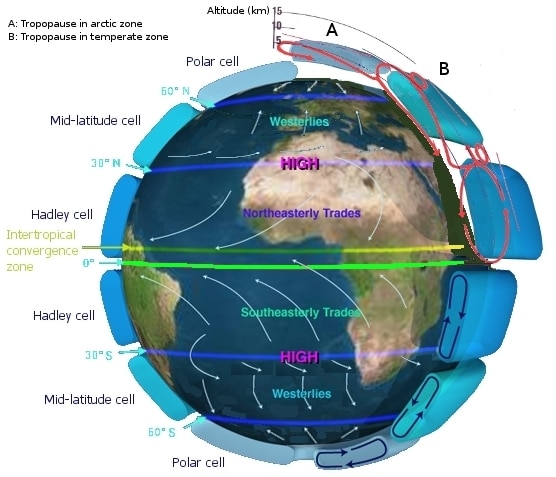
Understanding cloud feedbacks under climate change entails an understanding of how warming will affect water vapour and cloud distributions and their impact on the Earth’s radiation budget. At present, it seems possible that tropical circulation patterns may not greatly affect the tropically averaged radiation budget, whereas in mid-latitudes a decrease in storm frequency and an increase in storm intensity may reduce the reflection of solar radiation back into space and generate a positive feedback. Polar clouds are believed to exert a positive feedback that may account for 40% of the Arctic warming so a great deal depends on how such clouds will respond as sea ice melts and snow cover diminishes.
Vapour trails from high-flying aircraft, contrails, high in the troposphere reflect and thereby reduce incoming solar radiation. However, cirrus clouds spreading from the original trails may add to the greenhouse effect. In the US, cirrus clouds have been increasing by about 1% per annum. In contrast to the original trails the cirrus are believed to reflect less sunlight than the amount they trap, especially in winter and spring and could conceivably increase temperature slightly.
Precipitation
Global precipitation is more difficult to predictthanglobal temperature, precipitation being more variable spatially and because of the difficulties involved in measuring precipitation over oceanic areas. Global land valuesof precipitationdecreased in the 1940s and again between 1980 and 1995 and were at a maximum in the relatively cool years between 1950 and 1976 when El Niño events were sparse. Regions with Mediterranean-type climates are relatively limited in area and are likely to suffer from lower rainfall totals with any poleward shift in desert margins resulting from anthropogenic warming.
With global warming, rainfall in Spain is expected to diminish. Rainfall, especially in the spring months, is currently very much influenced by the North Atlantic Oscillation and this is likely to continue to be the case in the future. More frequent and more severe droughts would have important consequences for agriculture because of the importance of irrigation to the economy, and also for power supplies because 13% of the country’s electricity is currently generated by hydro power and higher temperatures would result in greater demands for air conditioning.
Volcanic Forcing
It is now well recognised that volcanic eruptions can produce negative radiation forcing as a result of the sulphate aerosols many of them project into the stratosphere. Knowledge of the scale of cooling has increased with the studies made of the successive eruptions of Agung (Indonesia) in 1965, El Chichón (Mexico) in 1982 and Pinatubo (Phillipines) in 1991. Ammann et al. (2003) argue that a combination of volcanic and solar forcing contributed to the early 20th century cooling prior to 1915 and to the late 20th century cooling after 1960. The latter could conceivably have been associated with the eruption of the Bezymianny volcano in Kamchatka in 1956: eruptions in high northern latitudes are more effective forcing agents than eruptions in low latitudes.
There seems to be a good correspondence over the last several hundreds of years between volcanic eruptions and cooling episodes. A greater understanding is now being obtained of the processes at work. Volcanic eruptions such as Krakatoa not only cool the ocean surface, thereby offsetting anthropogenic warming for a few years, but they also create a long-lasting thermal anomaly deep in the ocean (Gleckler et al., 2006). Such events may even affect the onset of El Niño (Kerr, 2003). Incidentally, the recent eruption of Eyjafjalljökull in Iceland has not had an important cooling effect as it has involved ash rather than sulphur.
An Australian geologist, Ian Plimer, in his provocative book heaven+earth (2009) which emphasises the need to include the effects of geological processes in the study of global warming, points to the possible importance of submarine volcanism as it affects the solute load and temperature of ocean waters. Ian Plimer’s book is deliberately provocative in its approach to the threat of climate warming. Submarine volcanism is one process he mentions as being important, because it involves the release of carbon dioxide and other gases soluble in sea-water and because it is also a heat source. Both are difficult to quantify. Great uncertainty is presented by our ignorance as to where and when eruptions will occur in the future and whether they will be more or less frequent than they have been so far in the Holocene.
Solar Radiation
It has been widely assumed that the Little Ice Age was associated with reduced solar radiation around 1700 when sunspots were absent during the Maunder Minimum and also during the Wolf (1280-1350) and Sporer (1450-1550) sunspot minima. Earlier reductions in solar radiation have been invoked to explain cooling at intervals of about 1,000 years in the Holocene indicated by the presence of glacial debris in North Atlantic sediments (Bond et al., 2001). Correlations have also been found between indications of lakes drying in the Jura and times of negative solar forcing (Magny, 1993).
The variation in solar radiation associated with the 11-year sunspot cycle has long been recognised, but is generally regarded as being on too small a scale to have a detectable effect on climate. Estimates of inter-decadal variations in solar forcing remain uncertain. They mainly involve variability of ultra-violet solar radiation interacting with stratospheric ozone possibly to give changes in the tropospheric circulation.
Over the last few years there has been a tendency for climatologists to revise the solar effects downwards. Solar forcing is now considered by the IPPC to be of the order of 0.2Wm-2, only one tenth that due to human activities. In support of this attitude Lockwood and Frochlich (2007, 2008) and Lockwood (2010) pointed out that while the sun’s output had declined for the last 20 years, temperatures on Earth had risen. Not all solar physicists agree. It still seems possible that early 20th century warming was the outcome of less volcanism and increased solar radiation and that the decrease in diurnal temperature range, especially in the 1970s, can be attributed to tropospheric aerosols and increased continental cloud cover. But it remains very likely, at least, that warming over the last 50 years has been caused by greenhouse gases.
Land-use Changes
The climatic effects of land use changes are not very well understood. Pielke et al. (2002) have suggested that the expansion of cropland and grazed land between 1700 and 1900 may well have played a part in global temperature rise over that period. The direct effects of increasing atmospheric CO2 on large-scale carbon uptake by plants and soils cannot be quantified at present. Afforestation in high northern latitudes and at higher altitudes in highland areas may increase the uptake of carbon dioxide but at the same time it is likely to reduce the albedo especially during the winter and spring seasons of snow cover (Betts, 2000). Deforestation in the tropics followed by burning and decomposition of the woody material and oxidation of the exposed soil, is usually taken to be an important source of increased CO2 in the atmosphere but studies using networks of atmospheric data demonstrate near-zero land atmospheric fluxes in the tropics, implying that tropical deforestation is currently approximately balanced by re-growth (IPCC 2007, Working Group 1 FAR, p. 528; Christenson et al., 2007). Tropical deforestation is likely to increase albedo and promote cooling but it could also increase carbon dioxide in the atmosphere and boost evaporation losses thereby increasing the water vapour content of the lower atmosphere and promoting warming.
The Cryosphere
The risk of coastal flooding as a result of ocean warming and seawater expansion plus the contribution of the cryosphere (glaciers and ice sheets) to ocean volume is one of the major threats of anthropogenic global warming. Glaciers and ice sheets respond to climate change relatively slowly, but because they are in remote regions they have been studied for only a limited time and so records are short, especially for Antarctica.
The ice-flow speed of Greenland glaciers south of 72o North is reported to have increased between 1990 and 2006 by up to 100%. The fronts of two east coast glaciers, Kangerdlugssuaq and Helheim, had been relatively stable for over 50 years but between 2002 and 2005, while the ice flow in their tongues accelerated, the fronts of both glaciers retreated more than 5km (Howat et al., 2007). Both the acceleration and the frontal retreat may be attributable to recent warm summers and both may point to a drawdown of the ice sheet. It has recently been found that outlet glaciers can respond rapidly to the occurrence of periods of warmer weather as a result of abundant melt water penetrating to the bed of the ice via moulins (see Glossary), allowing the ice to accelerate. Such movements may be short-lived and Howat et al. recognise that they should not be used as indicators of long-term trends.
In the Southern Hemisphere, sea ice around Antarctica has not been reduced to the same extent as sea ice in the Northern Hemisphere. On the other hand, shelf ice bordering the Antarctic continent, especially West Antarctica, is showing signs of disintegration. Melting of the shelf ice contributes little to sea level rise. The main concern is that its removal allows glaciers streaming from the ice cap to accelerate, thereby reducing the mass of land-based ice and contributing to sea-level rise.
Even a modest change in ice-sheet balance over Antarctica could strongly affect future sea level and freshwater flux to the ocean. It has been widely suspected that higher temperatures and greater water-vapour content of air moving over Antarctica might bring greater snowfall and a build-up of ice which would counteract the effect of greater melting at the margins. There is now more uncertainty that this will be the case.
Much attention has been attracted to the unfortunate inclusion of a comment in the 2007 IPCC report that read: ‘Glaciers in the Himalaya are receding faster than in any other part of the world and, if the present rate continues, the likelihood of them disappearing by the year 2035 and perhaps sooner is very high if the Earth keeps warming at the present rate’. Himalayan glaciers occupy a wider area than glaciers in any other region outside the polar regions. Their history is very uncertainly known, as there are practically no documentary records relating to their extent before the 19th century when officers of the Survey of India and various travellers made useful observations together with drawings and maps. There have been minor glacier advances from time to time but since 1880, and probably over the preceding century, glacier retreat has predominated (Grove 2004, pp. 229-47). There is no risk however of the glaciers disappearing within the next 25 years. On the other hand, snowmelt earlier in the year and glacier shrinkage as a result of warming is beginning to affect river discharges and this could affect water storage, causing problems for hundreds of millions of people who depend on Himalayan water for irrigating their crops, but the future of monsoon rainfall is equally important. Nevertheless, greater attention should certainly be paid to the past and present behaviour of the Himalayan glaciers.
Sea-level Rise
The rate of sea-level rise is known with high confidence to have increased from the mid-19th century to mid-20th century when the mean rate of rise was 1.7mm per year. By the end of the 20th century the rate of increase according to satellite observations was put at 3.1 ± 0.7mm per year. The IPCC in its Fourth Report (2007) predicts a rise of 18-38cm in its most optimistic scenario and a rise of 26-59cm in its most pessimistic. Even if greenhouse gas levels are stabilized the rate of rise is likely to continue to increase for some time.
Rates of rise vary regionally as a result of variations in ocean temperature change, salinity and wind effects. The largest rises have been in the Pacific and eastern Indian Ocean where future rises depend a good deal on ENSO. It is quite possible that the sea level could fall if snowfall over the ice sheets were to increase as a result of rising temperatures. Present trends suggest that sea level by the end of the century will be less than half a metre higher than now.
The Past, Present and Future of Climate Change
This section provides a quick review of past, present and future climate change, with a comprehensive view of the Earth’s climate history (including the recent past) as well as future climate predictions.
The Little Ice Age and the Medieval Warm Period
In the European Alps, the record of glacier advances and retreats in recent centuries is unusually well known from written accounts, artists’ paintings, maps and photographs as well as from geological studies. The record points to intervals within the last 700 years, each lasting several decades, when glaciers extended hundreds of metres further down their valleys than they do now. It has been called the Little Ice Age (see Glossary). The warming required to account for the retreat of Alpine glaciers from their most distant Little Ice Age moraines to their present positions is between 0.6º and 0.7oC, a value similar to that of global warming over the last 100 years (Broecker, 2005).
Figure 10. The Hunters in the Snow by Pieter Brueghel the Elder, 1565
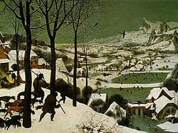
In Europe, the lowest temperatures of the Little Ice Age occurred within the interval 1645 to 1715 when it is known that sunspot activity was much reduced. It is called the Maunder Minimum (see Glossary). It has been proposed that the Little Ice Age was one of general global cooling but climate records are not good enough to warrant this assumption. It might be hoped that records of glacier advances would help to clarify the situation. However, it has been found that during the late Maunder Minimum (1675 to 1715), when sunspots were exceptionally rare and winters in Europe are known to have been exceptionally severe, glaciers in Switzerland failed to advance because winter snowfall there and in continental Western Europe generally over the 40-year interval was unusually deficient.
Figure 11.
Source: prepared by Robert A. Rohde, part of the Global Warming Art Project, http://en.wikipedia.org/wiki/Maunder_Minimum.
The question arises as to whether the Little Ice Age was a regional or a worldwide event. In 1992 Bradley & Jones published an account of climate since AD 1500 bringing together data from 29 regional studies. All except one were based on tree rings or ice cores. They demonstrated that the climate of the last 1,000 years was characterised by complex anomalies each lasting no longer than a few decades. No synchronous cold period was revealed but there were seen to have been at least two widespread cool periods in the last 1,000 years, one beginning about 1275 and the other around 1510. Within the latter, a few short cool episodes in the 1590s to 1610s, 1690s to 1710s, 1800s to 1810s and 1880s to 1900s were seen as synchronous on the hemispherical and global scale. Bradley & Jones concluded that the last 500 years had not experienced an overall cold period and that the coldest periods in one region were often not coincident with those in other regions.
Gordon Manley (1974) reconstructed temperatures in central England back from 1973 to 1659 by making use of information he assembled from a number of instrumental records and diaries. His results show, as one might expect, that there were fluctuations from one year to another and one decade to another. The coldest decade he identified is centred on 1700 in the middle of the Maunder Minimum when, Manley concluded, temperatures in central England were 2oC below the mean for the whole 314-year period.
Much documentary information is available in western and Mediterranean Europe relating to climate. The Spanish archives, which Martin-Vide, Barriendos, Rodrigo and others are beginning to exploit, have great potential for throwing light on climate history in medieval and later times, especially rainfall variability at different time scales. Guiot et al.(2005) have traced temperatures at Marseille from a variety of documentary evidence, notably grape-harvest dates from France and tree-ring information. They found temperatures were 0.5°C lower in the Little Ice Age with a maximum cooling of 1.5°C in phase with Western Europe. The decade with the coldest Mediterranean winter temperatures in the proxy-based reconstruction was 1680-1689.The coldest winter in the series, probably the coldest winter in Europe for at least half a millennium, was 1708/9 when the Venetian lagoon and canals froze.
The Medieval Warm Period of the 9th and 10th centuries is another instance of global climate within the historical period differing from that of the present day. This was the time when the Vikings voyaged to south-west Greenland and established settlements there that persisted into the 14th century, indicating that the sea-ice cover in the Arctic Ocean was less extensive than it was to be in later centuries. Twelfth century coastal flooding around the North Sea suggests that the sea level may have been 20cm higher than today. Place names and written records in parts of north-western Europe indicate that vines were being grown further north in early medieval times than in the Little Ice Age. However, grape-harvest dates in France suggest that mean temperatures never exceeded those of the present day for any considerable length of time and it is possible that the disappearance of vineyards from northern lands in later medieval times was the result of the development of a sea-borne trade in wine rather than climate cooling.
A more precise item of evidence comes from Switzerland, where Holzhauser (1984) has traced the history of an aqueduct constructed near the Grosser Aletsch glacier around 1200 AD to bring water to an Alpine village. The aqueduct is known to have been destroyed when the glacier advanced in 1240 AD, an event that may be regarded as marking the end of the Medieval Warm Period.
In China, phenological evidence that crop boundaries lay further north in the 12th and early 13th centuries than in the late 20th century has been provided by Zhang De’er (1994). Generally, however, spatial coverage, temporal resolution and age control of most of the available data, such as that presented by Grove & Switsur (1994) are insufficient to determine if there were multidecadal periods of global warmth during medieval or other times in the Holocene on a scale similar to the global warming that has taken place since 1980.
Studies such as those mentioned above are important in connection with present uncertainties about global warming, because many sceptics are inclined to point to the Little Ice Age and the Medieval Warm Period as indicating that before the industrial revolution global temperature varied quite naturally by as much as it is known to have varied since carbon dioxide concentrations in the atmosphere increased, and they prefer to regard global warming over the last three decades as just a natural fluctuation.
Uncertainties continue to exist about the Holocene climatic record and the range through which global temperatures fluctuated over the last 10,000 years. That there were fluctuations is undoubted, but they may have been limited in extent to individual regions or to one Hemisphere. In its Third Assessment Report, the IPCC accepted that there were widespread cooler conditions in the 12th, 14th, 17th and 19th centuries but accorded less credence to the evidence for a widespread Medieval Warm Period. In the context of the last half millennium, it seems likely that the last three winter decades have been the warmest and driest.
Recently, sources of information about Holocene climate that have become available include borehole records from all the continents[7]. They do not permit annual or decadal resolution but the data go back more than 20,000 years. They show the last glacial maximum (see Glossary), a mid-Holocene warm episode, the Medieval Warm Period, the Little Ice Age and the rapid warming of the 20th century (Huang et al. 2008). Except for the last of these, the fluctuations in temperature are not explicable in terms of human activity. But the borehole data are not sufficiently precise to determine whether the temperature variations they indicate were as great as those that are known to have taken place in the last 160 years according to the instrumental records.
Climate Since the Last Glacial Period
The continental ice sheets reached their maximum extent between 27,000 and 19,000 years ago, largely in response to a decrease in northern summer insolation associated with precession (the motion of the Earth’s axis, resembling that of a spinning top with its axis sweeping out a cone). At the same time sea surface temperatures in the tropical Pacific were low, and so were values of atmospheric CO2 (Clark et al., 2009). Subsequent deglaciation of the Northern Hemisphere is believed to have been induced by an increase in northern summer insolation, increasing concentrations of atmospheric CO2 and an abrupt rise in sea level.
As mentioned above, the end of the Last Glacial Period of the Pleistocene Ice Age in the Northern Hemisphere is marked by the Younger Dryas (see Glossary), which the ice-core record shows to have been a short, sharp cold interval lasting from 12,800 to 11,200 years ago. Early Holocene warmth following the Younger Dryas was interrupted around 8,500 years ago by a widespread cooling in the Northern Hemisphere lasting about seven centuries which, like the Younger Dryas, was probably caused by an enormous eruption of fresh water into the north-western Atlantic Ocean from beneath and around the decaying North American ice sheet interrupting the Thermohaline Circulation of the world’s oceans. The cooling event about 8,500 years ago was followed in the Northern Hmisphere by the Mid-Holocene warm episode that lasted until about 5,000 years ago.
Figure 12. The Younger Dryas Period
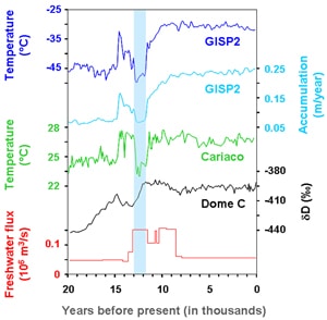
Source: Timmer (2009), http://arstechnica.com/science/news/2009/01/an-impact-for-the-younger-dryas-extinction.ars.
During the Early Holocene and the Mid-Holocene warm periods, the Earth was nearer the sun during the northern summer than it is now, because of precession (see Glossary), and as a result the monsoon was stronger. With heavier monsoon rains extending further north than they do now, an enormous lake, Megachad, similar in size to the Caspian Sea of the present day, occupied a large part of the south-east Sahara. It was fed by rivers from Darfur and Tibesti as well as from the equatorial regions to the south. The presence of such a lake must itself have modified the local climate. Elsewhere in tropical Africa, and also in northern India, lake levels were tens of metres higher than they are at the present day.
Figure 13. Physiographic setting of the Chad Basin
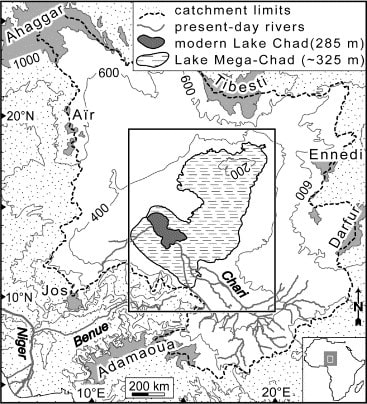
Figure 14. Shaded relief image derived from the SRTM30 DEM of the Chad Basin, highlighting Holocene Lake Mega-Chad shoreline features
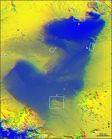
Source: Schuster, Roquin, Brunet, Duringe, Caugy, Fontugne, Taïsso, Vignaud, & Ghienne (2005), ‘Holocene Lake Mega-Chad Palaeoshorelines from Space’, Quaternary Science Reviews, vol. 24, nr 16-17, September, p. 1821-1827.
The ancient shore of Megachad can be easily recognised on satellite imagery. Much of the old lake floor, especially the Bodélé Depression at the lake floor’s lowest level, is today carpeted white by diatomite (see Glossary), the microscopic remains of algae that lived in the ancient lake. North-easterly winds, constricted into a low level jet by the Tibesti Mountains to the north, drive sand over the desert surface, abraiding the diatomite and at times creating a fog to the west and south of Tibesti. The finest dust is transported to the coastal areas of West Africa where it is partly responsible for the Harmattan (see Glossary) haze from November to April. Some of the dust eventually settles in the Atlantic and even as far away as the Amazon basin. It is suspected that the floor of Megachad is one of the most important global sources of atmospheric dust and the aerosols may have a significant effect on global climate over a very wide area.
Holocene Climate Change
In spite of the IPCC reports and the weight of scientific opinion that acknowledges greenhouse gases are responsible for current global warming, there are still many who are unconvinced that this is the case. They believe that the warming since the nadir of the Little Ice Age, between about 1680 and 1710, is within the range of natural variability. They also point to the fact that temperatures began to rise before greenhouse gas concentrations had increased on account of high rates of fossil-fuel usage, neglecting to recognise that carbon dioxide was being released in the 19th century by forest clearance and soil tillage in North America, Siberia and Australia and by draining peat bogs in Europe.
Predicting Future Global Temperature
Uncertainty as to the rate at which global temperatures will rise as a result of the increasing concentrations of carbon dioxide in the atmosphere is likely to persist for a variety of reasons. The value of about 3°C given by the IPCC as the sensitivity to a doubling of carbon dioxide is the same as that given to the US National Academy of Sciences in 1979 by Jule Charney when he was head of a study group which assessed the scientific basis for the projection of possible future climate change resulting from anthropogenic carbon dioxide emissions.
Charney’s group did not examine the role of the biosphere or the workings of the world economy in the carbon cycle. However, it did recognise the importance of the positive feedback mechanism of the increase in moisture and also the negative feedback of increased cloud amount and it pointed to a possible delay in warming on account of the time taken for thermal equilibrium to be established in the surface and intermediate layers of the ocean. Charney’s report concluded that ‘the predictions of CO2 induced climate changes made with the various models are basically consistent and mutually supporting. The differences in model results are relatively small and may be accounted for by differences in model characteristics and simplifying assumptions. Of course, we may never be sure that some badly estimated or totally overlooked effect may not vitiate our conclusions. We can only say that we have not been able to find such effects. If the CO2 concentration of the atmosphere is indeed doubled and remains so long enough for the atmosphere and the intermediate layers of the ocean to attain approximate thermal equilibrium, our best estimate is that changes in global temperature of the order of 3°C will occur and that these will be accompanied by significant changes in regional economic patterns’.
Charney, in 1979, was unaware that there were other greenhouse gases that had to be taken into account, the most important being ozone O3 and methane CH4. Nevertheless, his assessment has been confirmed in general terms by later studies. Research on climate change science at the Hadley Centre (UK Meteorological Office) predicted in 2004 that the most likely global average temperature rise for a doubling of the concentration of atmospheric carbon dioxide was 3.5°C, with a 90% probability that the warming will be between 2.4°C and 5.4°C. The full range (ie, scenario plus climate model range) of 1.4°C to 5.8°C is a much-cited finding of Working Group One in the IPCC’s Third Assessment Report but the lack of discussion of associated likelihood in the report made the interpretation and useful application of this result difficult. In Chapter 2 of Working Group One in the Fourth Assessment Report, the range of 1.5°C to 4.5°C is given for climate sensitivity to atmospheric CO2 doubling, but with no confidence assigned.
Roe & Baker (2007) inquired into why uncertainties in the projections of future climate sensitivity have not lessened substantially over the past 30 years in spite of increased efforts and tremendous increases in computing power. In particular, they pointed to the long tail in probability distributions of small but finite probabilities of very large temperature increases and concluded that the uncertainty of climate sensitivity is ‘a direct and general result of the fact that the sum of the underlying climate feedbacks is substantially positive’.
The 5% possibility that global temperature change for a doubling of CO2 may exceed 4.5°C is not something that can be ignored. An increase in global temperatures of 2°C or 3°C would have important consequences (especially in high northern latitudes where the rise in temperature would be greater) but if it were to take place steadily and slowly would allow economic and other adjustments to take place that might reduce the impact. On the other hand, greater global warming, especially if it were to take place rapidly, as it would inevitably do in some regions, especially the Arctic, could conceivably be much more serious in its consequences. The uncertainty is therefore of much importance.
Future Changes in Greenhouse Gas Concentrations
Future changes in greenhouse gas concentrations and global temperature depend on many factors, among which the most important are the rate at which the burning of fossil fuels and the manufacture of cement continue and the success or not of burying or otherwise sequestrating greenhouse gas emissions. The prospects are not very encouraging. Politicians in most countries find themselves unable to take unpopular measures and their electorates are inclined to put personal fulfilment before public well-being. Expansion of the economies of China, India and other South-East Asian countries is unlikely to slow down significantly for many years, and western countries are unlikely to yield economic leadership willingly. With populations concentrating in urban areas, cement-making is unlikely to diminish. Burial of greenhouse gases is expensive and not possible everywhere. Renewable sources of energy are not readily exploited.
Atmospheric CO2 growth exhibits large interannual variability associated with ocean-atmosphere variability in the Pacific and further afield. High rates of growth correspond to El Niño (see Glossary) and are often accompanied by droughts, higher temperatures and forest fires. Lower rates correspond with La Niña[8] (see Glossary), generally accompanied by higher rainfall and somewhat lower temperatures. In the early 1990s, when there was a modest El Niño, lower temperatures caused by Pinatubo aerosols scattering sunlight reduced soil respiration and enhanced Northern Hemisphere carbon uptake. Surface waters were cooled and sank, taking CO2 down into the ocean.
Deforestation has been responsible for CO2 growth in the past and it is likely to continue for many years in the tropics. However, in much of Europe and the US forests and woodlands increased in the 20th century. Even in Amazonia, much CO2 emission from logging and clearing is compensated by uptake with re-growth of vegetation. There is a possibility that increased atmospheric CO2 will result for a time in higher rates of uptake by growing plants. On the other hand, if soil water becomes less available as a result of greater evaporation losses or lower rainfall, net primary production and uptake of CO2 by plants may be reduced. Drier conditions could result in more forest fires, increasing CH4 and CO2 emissions, as in the 1998 El Niño period. There is still much uncertainty about the flux of CO2 released to the atmosphere by land-use changes and the take-up by the oceans.
Regional and Short-term Climate Change
Global climates are evidently set to warm on account of the high and continually increasing concentrations of greenhouse gases in the atmosphere. While global temperature appears to have varied remarkably little in the course of the Holocene, there have been important regional changes in temperature and precipitation. In the future, warming will not increase regularly because of the varying influence of other forcing factors, notably El Niño events, which accentuate warming and powerful volcanic eruptions, which are negative. Either is capable of counteracting greenhouse warming for several years. Uncertainty about short-term regional and short-term climate change is consequently much greater than uncertainty about long-term global change.
Although long-term global change eventually affects everyone, over the next decade or two, regional shorter-term changes are likely to affect the individual country and the individual citizen more severely. It can be argued that, in the short term, El Niño and ENSO are more important to people than anthropogenic global climate change. Other important influences on regional climate are various oscillations of atmospheric pressure, notably the North Atlantic Oscillation, the Northern Annular Mode, the Southern Annular Mode, the Pacific-North American pattern, the Pacific Decadal Oscillation and the Indian Ocean Dipole (see Glossary). Much depends on how these systems, which are highly influenced by sea surface temperatures, respond to global warming. At present the impact of global warming on the performance of ENSO and the other Oscillations and consequently on regional and short term climate change is very uncertain.
Partly as a result of regional climatic variability, global temperatures vary from year to year and will continue to do so, possibly in an unpredictable way, while long-term mean values, say 50-year means, steadily rise. In other words, although global warming in the long term is certain so long as greenhouse gas emissions remain high, in the short-term global temperature change from year to year is uncertain. This is exemplified by the fact that peak annual global temperatures were reached in 1998 and 2005 whereas temperatures were lower between those dates and have been lower since 2005.
Climate changes have been more apparent in the land areas of the Northern Hemisphere than they have been in the oceans and the Southern Hemisphere. In the course of the Holocene it appears that warming in one hemisphere has been balanced by cooling in the other. The early Holocene saw warming in high northern latitudes and the expansion polewards of boreal forest. This warming coincided with the greening of the Sahara and higher lake levels throughout Africa north of the Equator. It included the expansion of Megachad over some 350,000km2 of Chad and Sudan between 10,000 and 6,000 years BP (see Glossary). These departures from present conditions can be explained in terms of precession (see Glossary), the Earth having been nearer the sun during the Northern Hemisphere summer than it was to be later in the Holocene and the northern summer monsoonal rains having been heavier than they are now and extending further north. In the near future, it may be expected that fluctuations in climate on a regional scale will be much greater than global climate changes.
Figure 15. Diagram of the Earth’s precession
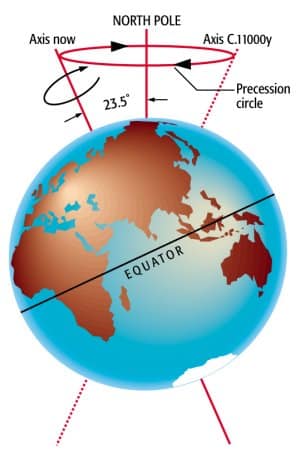
Late 20th century Arctic warming has been replicated in all models and, in fact, winter Arctic ice extent has decreased over the last 30 years by 4% per decade. It was predicted that Arctic sea ice would disappear in September by the end of the 21st century. But changes have taken place more rapidly than expected. By September 2007 the North Pole was free of sea ice and the total area of Arctic sea-ice was only 4.28 million sq km. A still smaller area of sea ice was expected for September 2008 but according to the National Snow and Ice Data Centre, University of Colorado, the area increased slightly that year to 4.67 million sq km and increased again in September 2009 to 5.36 million sq km. It is now suspected that wind effects played an important part in the 2007 diminution. Masayo Ogi et al. (2010) have shown that the combined effect of winter and summer wind forcing accounts for 50% of the variance of the change in September Arctic sea-ice extent from one year to the next, with anomalies in the meridional wind to the north and east of Greenland modulating the export of ice through the Fram Strait. Meanwhile, in recent decades, the area of Antarctic sea-ice has been slightly increasing.
Precipitation is even more difficult to predict on a regional scale than temperature. An entirely satisfactory explanation for the Sahelian drought of the 1970s and 1980s is still wanted. It seems likely that it was related to low sea-surface temperatures in the Indian Ocean and possibly the Atlantic.It has also been suggested that industrial aerosol pollution from Europe and North America affected properties of clouds in the Northern Hemisphere causing them to reflect more sunlight back into space, thereby cooling the northern oceans and prompting tropical rain bands to move south, tracking away from the more polluted Northern Hemisphere.
In the 19th century the strength of the South Asian monsoon was dominated by the influence of El Niño. In the latter part of the 20th century the correlation of monsoon strength and El Niño was much less and Indian Ocean temperature and atmospheric pressure distribution have exerted more influence. The Indian Ocean Dipole (see Glossary) has at the same time exerted an influence over east African rainfall and to a lesser extent Ethiopian rainfall, notably in 1961.
Predictions are that high northern latitudes are likely to receive more precipitation and low latitudes less as a result of anthropogenic warming, but the situation varies from one region to another. The existing ocean currents, stratospheric jet streams and large-scale oscillations of atmospheric pressure are expected to continue to influence regional climates. There seems to have been a change in ENSO and Pacific climate generally in 1976-7 and the strength and periodicity of such phenomena in the future may well differ from the present (IPCC Fourth Assessment, Working Group 1, p. 288-9).
Concluding Remarks
This paper has attempted to summarise the state of present knowledge relating to uncertainty in climate change. So far as policy implications are concerned, the COP16 meeting is the next item on the agenda. As this Working Paper argues, uncertainty is inherent in climate change and, furthermore, different types of uncertainty co-exist. For policy makers this can be either a motivation for action, or an excuse for inaction.
The Paper concludes that despite inherent uncertainty, evidence is increasing that human activity is causing global warming. Even if it were to be proved at a later stage that there are other explanations, it is safer to act, to mitigate and adapt with the aim of slowing down change. This would buy more time for knowledge to increase (Webster et al., 2003) and for the means to be discovered for decarbonising economic activity.
The biggest current challenge would now seem to be in predicting regional climate change, since it is expected that regional departures from present precipitation and temperature means and extremes will exceed global departures. This is an area where science and policy should go hand in hand, to insert uncertainty about regional climatic change into current policy decisions. In relation to this uncomfortable interface between science and policy, it is important to consider that ‘among several ways of reacting to or anticipating climate changes invokes genuine moral values that science can –and indeed should– be neutral about… scientific, i.e. climatological or economical, prognoses as regards climate change… taken on their own, give no sufficient reasons for acting or not acting, this way or the other’ (Hillerbrand & Ghil, 2008, p. 2136).
In terms of political decisions, actions to mitigate climate change are subject to moral choices that will probably always operate in the context of inescapable climatic uncertainty.
A.T. Grove
Emeritus Fellow of Downing College, University of Cambridge
E. Lopez-Gunn
Senior Research Fellow, Water Observatory-FMBotín and Visiting Senior Fellow, LSE
Bibliographical References
Ammann, C.M., G.A. Meehl, W.M. Washington, C.S. Zender (2003), ‘A Monthly and Latitudinally Varying Volcanic Forcing Dataset in Simulations of 20th Century Climate’, Geophysical Research Letters, nr 30, p. 1657.
Betts, R.A. (2000), ‘Offset of the Potential Carbon Sink from Boreal Forestation by Decreases in Surface Albedo’, Nature, nr 408, p. 187.
Birks, H.H., W. Eide & H.J.B. (1999), http://www.sciencemag.org/cgi/content/full/286/5446/1815a.
Bloom, A., P.I. Palmer, A. Fraser, D.S. Reay & C. Frankenberg (2010), ‘Large-scale Controls of Methanogenesis Inferred from Methane and Gravity Spaceborne Data’, Science, nr 327, p. 322-5.
Bond, G., B. Kromer, J. Beer, R. Muscheler, M.N. Evans, W. Showers, S. Hoffmann, R. Lotti-Bond, I. Hajdas & G. Bonani (2001), ‘Persistent Solar Influence on North Atlantic Climate During the Holocene’, Science, nr 294, p. 2130-6.
Bradley, R.S., P.D. Jones (1992), ‘Climate since AD 1500’, Routledge, London.
Broecker, W.S. (1989), ‘Routing of Meltwater from the Laurentide Ice Sheet during the Younger Dryas Cold Episode’, Nature, nr 341, p. 318-21.
Broecker, W.S. (2004), ‘Future Global Warming Scenarios’, Science, nr 304, p. 388.
Broecker, W.S., & T.F. Stocker (2006), ‘The Holocene CO2 Rise: Anthropogenic or Natural?’, EOS, nr 87, p. 27-8.
Brooks, C.E.P. (1926), Climate Through the Ages, Benn, London.
Callendar, G.S. (1938), ‘The Artificial Production of Carbon Dioxide and its Influence on Climate’, Quarterly Journal Royal Meteorological Society, nr 64, p. 223-40.
Charney, J. (1979), ‘Carbon Dioxide and Climate: A Scientific Assessment’, Report of an Ad Hoc Study Group on Carbon Dioxide and Climate, Woods Hole, Massachusetts, National Academy of Sciences, Washington DC, http://www.atmos.ucla.edu/~brianpm/download/charneyreport.pdf.
Christensen, J.H., B. Hewitson, A. Busuioc, A. Chen, Gao X, Held I, Jones R, Kolli RK, Kwon W-T, Laprise R, Magaa Rueda V, Mearns L, Menndez CG, Risnen J, Rinke A, Sarr A, Whetton P (2007) Regional Climate Projections. Climate Change 2007: The Physical Science Basis. In: Contribution of Working Group I to the Fourth Assessment Report of the Intergovernmental Panel on Climate Change [Solomon S, Qin D, Manning M, Chen Z, Marquis M. Averyt KB, Tignor M and Miller HL (eds.)]. Cambridge University Press, Cambridge, United Kingdom and New York.
Clark, P.U., A.S. Dyke, J.D. Skakun, A.E. Carlson, J. Clark, B. Wohlfarth, J.X. Mitrovica, S.W. Hostetler & A.M. McCabe (2009), ‘The Last Glacial Maximum’, Science, nr 325, p. 710-4.
Etheridge, D.M., L.P. Steele, R.L. Langenfelds, R.J. Francey, J.M. Barnola & V.I. Morgan (1996), ‘Natural and Anthropogenic Changes in Atmospheric CO2 over the Last 1,000 Years from Air in Antarctic Ice and Firn’, Journal Geophyical Research, nr 101, D2 4115-28.
Eyet et al. (2004), ‘Comparison of two 13 CO2 records measured on air from the EPICA Dome C and Kohnen Station Ice Cores’, European Geophysical Abstracts, nr 6, ECU04-A-01990.
Farman, J.C., B.G. Gardiner & J.D. Shanklin (1985), ‘Large Losses of Total Ozone in Antarctica Reveal Seasonal C10x/NOx Interaction’, Nature, nr 315, p. 207-10.
Gleckler, P.J., T.M.L. Wigley, B.D. Santer, J.M. Gregory, K. AcutaRao & K.E. Taylor (2006), ‘Krakatoa’s Signature Persists in the Ocean’, Nature, nr 439, p. 675.
Grove, J.M. (2004), Little Ice Ages Ancient and Modern, vol. 1, 2nd edition, Routledge, London & New York, p. 229-47.
Grove, J.M., and R. Switsur (1994), ‘Glacial Geological Evidence for the Medieval Warm Period’, Climatic Change, nr 26, p. 143-69.
Guiot, J., A. Nicaut, C. Rathgeber, J.L. Edouard, F. Gulbal, G. Pichard & C. Till (2005), ‘Last-millennium Summer-temperature Variations in Western Europe Based on Proxy Data’, The Holocene, nr 15, p. 489-500.
Hillerbrand, R., & M. Ghil (2008), ‘Anthropogenic Climate Change: Scientific Uncertainties and Moral Dilemmas’, Physica, D 237, p. 2132-38.
Holzhauser, P. (1984), ‘Rekonstruktion von Gletscherschwankungen mit Hilfe Fossiler Holzer’, Geographia Helvetia, nr 39, p. 3-15.
Howat, I.M., I. Joughin & T. Scambos (2007), ‘Rapid Changes in Ice Discharge from Greenland Outlet Glaciers’, Science, nr 315, p. 1559-61.
Indermühle, A., T.F. Stocker, F. Joos, H. Fischer, H.J. Smith, M. Wahlen, B. Deck, D. Mastrolanni, J. Tschumi, T. Blunier, R. Meyer & B. Stauffer (1999), ‘Holocene Carbon-cycle Dynamics based on CO2 Trapped in Ice at Taylor Dome, Antarctica’, Nature, nr 398, p. 121-6.
Keeling, C.D., & T.P. Whorf (2005), ‘Atmospheric CO2 Records from Sites in the SIO Air Sampling Network. Trends: A Compendium of Data on Global Change’, Carbon Dioxide Information Analysis Center, Oak Ridge National Laboratory, US Department of Energy, Oak Ridge, Tenn.
Kerr, R.A. (2003), ‘Volcanic Blasts Favor El Niño Warmings’, Science, nr 299, p. 336-7.
Lerner, K. Lee, & Brenda Wilmoth Lerner (Eds.) (2003), ‘El Niño and La Niña Phenomena’, World of Earth Science, Gale Cengage, eNotes.com, 2006, accessed 28/V/2010, http://www.enotes.com/earth-science/el-nino-la-nina-phenomena.
Lionello, P., P. Malanotte-Rizzoli & R. Boscolo (Eds.), ‘Mediterranean Climate Variability’, Developments in Earth & Environmental Sciences, nr 4, http://www.climate.unibe.ch/~casty/med_book2005.pdf.
Lockwood, M. (2010), ‘Solar Change and Climate: An Update in the Light of the Current Exceptional Solar Minimum’, Proceedings of the Royal Society, A 466, p. 303-29.
Lockwood, M., & C. Frohlich (2007), ‘Recent oppositely-directed trends in solar climate forcings and the global mean surface air temperature’ Proceedings of the Royal Society, A 463, p. 2447-60.
Lockwood, M., & C. Frohlich (2008), ‘Recent Oppositely Directed Trends in Solar Climate Forcings and the Global Mean Surface Air Temperature. II. Different Reconstructions of the Total Solar Irradiance Variation and Dependence on Response Time Scale’, Proceedings Royal Society London, A 464, p. 1367-85.
Lorenz, E.N. (1963), ‘Deterministic Nonperiodic Flow’, Journal of the Atmospheric Sciences, nr 20, p. 130–141.
Magny, M. (1993), ‘Solar Influences on Holocene Climatic Changes Illustrated by Correlations between Past Lake-level Fluctuations and the Atmospheric 14C Record’, Quaternary Research, nr 40, p. 1-9.
Manley G. (1974), ‘Central England Temperatures: Monthly Means 1659 to 1973’, Quarterly Journal of the Royal Meteorological Society, nr 100, p. 389-405.
Mann, M.E., R.S. Bradley, M.K. Hughes (1998), ‘Global-scale Temperature Patterns and Climate Forcing over the Past Six Centuries’, Nature, nr 392, p. 779-787.
Masayo Ogi, Koji Yamazaki & J.M. Wallace (2010), ‘Influence of Winter and Summer Surface Wind Anomalies on Summer Arctic Sea Ice Extent’, Geophysical Research Letters, March, vol. 37.
McKitrick, R.R., P.J. Michaels (2007), ‘Quantifying the Influence of Anthropogenic Surface Processes and Inhomogeneities on Gridded Surface Climate Data’,Journal of Geophysical Research-Atmospheres 112, D4S09, doi:10.1029/2007JD008465.
Mercer, J.H. (1978), ‘West Antarctic Ice Sheet and CO2 Greenhouse Effect: A Threat of Disaster’, Nature, nr 271, p. 321-5.
Mestre, A. (2008), ‘Perspectivas y Retos: Planificación y Cambio Climático’, Colegio de Ingenieros de Caminos, Canales y Puertos Madrid, Madrid, 19-20/XI/2008.
Monnin, E., U. Siegenthaler, K. Kawamura, B. Bellier, J.M. Barnola, B. Stauffer, T.F. Stocker (2003), ‘Holocene CO2 Records from the EPICA Dome C and Kohnen Station (DML) Ice Cores’, Geophysical Research Abstracts, nr 5, p. 10775.
Murton, J.B., M.D. Bateman, S.R. Dallimore, J.T. Teller, Zhirong Yang (2010), ‘Identification of Younger Dryas Outburst Flood Path from Lake Agassiz to the Arctic Ocean’, Nature, nr 464, p. 740-3.
NASA (2010) http://earthobservatory.nasa.gov/Features/Clouds.
National Snow and Ice Data Center, University of Colorado, Boulder, Colorado, http://nsidc.org/sotc/sea_ice.html.
Neftel, A., E. Moor, H. Oeschger & B. Stauffer (1985), ‘Evidence from Polar Ice Cores for the Increase in Atmospheric CO2 in the Past Two Centuries’, Nature, p. 315, p. 45-47.
Oerlemans, J. (2005), ‘Extracting a Climate Signal from 169 Glacier Records’, Science, nr 308, p. 675-7.
Pielke, R.A., G. Marland, R.A. Betts, T.N. Chase, J.L. Eastman, J.O. Niles, D.S. Niyogi & S.W. Running (2002), ‘The Influence of Land-use Change and Landscape Dynamics on the Climate System: Relevance to Climate-change Policy Beyond the Radiative Effect of Greenhouse Gases’, Philosophical Transactions Royal Society London A, p. 360, p. 1705-19.
Plimer, I. (2009), heaven+earth, Global Warming: The Missing Science, Connor Court, Ballan, Australia.
Ramanathan, V., & G. Carmichael (2008), ‘Global and Regional Climate Changes Due to Black Carbon’, Nature Geoscience, nr 1, p. 221-7.
Revelle, R., & H.E. Suess (1957), ‘Carbon Dioxide Exchange between Atmosphere and Ocean and the Question of an Increase of Atmospheric CO2 During the Past Decades’, Tellus, nr 9, p. 18-27.
Roe, G.H., & M.C. Baker (2007), ‘Why is Climate Sensitivity so Unpredictable?’, Science, nr 318, p. 629-36.
Ruddiman, W.F. (2003), ‘The Anthropogenic Greenhouse Era Began Thousands of Years Ago’, Climatic Change, nr 61, p. 261-93.
Ruddiman, W.F. (2007), ‘The Early Anthropogenic Hypothesis: Challenges and Responses’, Reviews of Geophysics, nr 45.
Ruddiman, W.F., Zhengtang Guo, Xin Zhou, Hanbin Wu & Yangan Yu (2008), ‘Early Rice Farming and Anomalous Methane Trends’, Quaternary Science Reviews, nr 27, p. 1291-5.
Schneider, S.H. (1989), ‘Greenhouse Effect: Science and Policy’, Science, nr 243, p. 771-81.
Shakhova, N., I. Semiletov, A. Salyuk, V. Yusupov, D. Kosmach & O.Gustafsson (2010), ‘Extensive Methane Venting to the Atmosphere from Sediments of the East Siberian Arctic Shelf’, Science, nr 327, p. 1246-50.
Shindell, D.T., G.A. Schmidt, R.L. Miller, M.E. Mann (2003), ‘Volcanic and Solar Forcing of Climate Change During the Preindustrial Era’, Journal of Climate, nr 16, p. 4094-4107.
Solomon, S., K.H. Rosenlof, R.W. Portmann, J.S. Daniel, S.M. Davis, T.J. Sanford, G.K. Plattner (2010), ‘Contributions of Stratospheric Water Vapour to Decadal Changes in the Rate of Global Warming’, Science, nr 327, p. 1219-23.
Stott, P., & J. Kettleborough (2002), ‘Origins and Estimates of Uncertainty in Predictions of Twenty-first Century Temperature Rise’, Nature, nr 416, p. 719-23.
Thompson, D.W.J., J.J. Kennedy, J.M. Wallace & P.D. Jones (2008), ‘A Large Discontinuity in the Mid-twentieth Century in Observed Global Mean Surface Temperature’, Nature, nr 453, p. 646-9.
Schneider, S. (2004), ‘Abrupt Non-linear Climate Change, Irreversibility and Surprise’, Global Environmental Change, nr 14, p. 245-58.
Travis, W. (2010), ‘Going to Extremes: Propositions on the Social Response to Severe Climate Change’, Climatic Change, nr 98, p. 1-19.
Wagner, F., S.J.P. Bohncke (1999), ‘Century-scale Shifts in Early Holocene Atmospheric CO2 Concentration’, Science, nr 286, p. 1971-73.
Wagner, F., B. Aaby & H. Visscher (2002), ‘Rapid Atmospheric CO2 Changes Associated with the 8,200-years-BP Cooling Event’, Proceedings National Academy Science USA, nr 99, p. 12,011-4.
Webster, M., C. Forest, J. Reilly, M. Babiker, D. Kicklighter, M. Mayer, R. Prinn, M. Sarofim, A. Sokolov, P. Stone & C. Wang (2003), ‘Uncertainty analysis of climate change and policy response’, Climatic Change, nr 61, p. 295-320.
Zhang De’er (1994), ‘Evidence for the existence of the Medieval Warm Period in China’, Climatic Change, nr 26, p. 289-97.
Annex 1: Global Temperature and Precipitation
The circulation of the Earth’s atmosphere is driven by solar energy. The sun is very much hotter near the core than in its outer layers and, as a result, it emits radiation at both high and low frequencies, from shortwave ultraviolet (UV) through the short-wave (SW) visible spectrum to long-wave infrared (LW).[9] The amount of short-wave radiation that reaches the top of the Earth’s atmosphere has a value of 1370Wm-2 (watts per square metre), the amount varying slightly from season to season because of the elliptical shape of the Earth’s annual orbit round the sun, and also varying from year to year and decade to decade according to the number of sunspots.
Figure 16. Sunspot activity
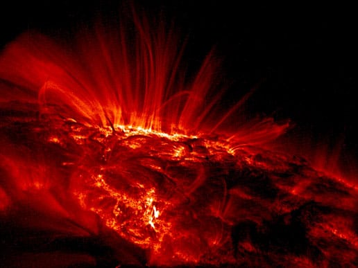
Figure 17. The sunspot cycle
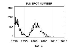
On average about 30% of the energy reaching the top of the Earth’s atmosphere is reflected back into space by clouds and by highly reflective surfaces such as the oceans, sea ice and ice sheets. Some of the photonscomprising the sunlight are absorbed by nitrogen and oxygen molecules and re-emitted at the same frequency as the original, moving off in any and every direction so that the overall effect is to give the sky its bright appearance. On a cloudy day there may be no direct sunlight, only diffuse lighting that fails to cast a shadow.
The amount of short-wave radiation an area receives depends first on its latitude. The axis of the Earth is tilted at an angle of 66.5o to the plane of the elliptical path it follows round the sun in the course of the year. On Northern Hemisphere Midsummer’s Day the sun is vertically overhead at midday at 23.5o N, on the Tropic of Cancer; on Southern Hemisphere Midsummer’s Day it is vertically overhead at midday at 23.5o S, on the Tropic of Capricorn. Throughout the year it is vertically overhead somewhere between the tropics, so that intertropical latitudes receive far more shortwave radiation than any other region.
The amount of short-wave radiation reaching a square metre of the Earth’s surface depends mainly on its latitude, on the amount of cloud and on the slope angle and direction of slope of the surface. The short-wave energy absorbed by the Earth’s surface warms it up. As a result, the surface emits long-wave, infrared radiation that is readily absorbed by clouds and also by three gases in the atmosphere, namely water vapour, carbon dioxide and methane. The clouds and the gases re-emit long-wave radiation but most of this energy stays in the lower troposphere, the lower part of the atmosphere. Because clouds are great absorbers and emitters of long-wave radiation, they act as blankets and, especially at night, they keep the surface several degrees warmer than it would be if the clouds were not there.
Since the troposphere is heated from the ground up, temperature decreases with height above the surface, at a rate of between 4o and 10oC per 1,000m. If the rate of cooling with height –the lapse rate (see Glossary)– is less than 9oC per 1,000m the air is likely to be stable, without a tendency to rise; if the lapse rate is more than 9oC per 1,000m the air tends to rise and is said to be unstable. As a parcel of unstable air rises and cools at the environmental lapse rate of around 9.8oC per 1,000m, it becomes saturated with water vapour. The water vapour condenses on very small ice crystals or other very fine particles, aerosols, to form water droplets and as it does so it releases heat, clouds form, the saturated adiabatic lapse rate declines to only about 6.5oC per 1,000m, the water droplets grow in size until they fall to Earth as rain, or freeze and fall as snow, and the air mass becomes more stable. Air also rises and cools and clouds form where air is forced to move upward as a result of crossing mountain ranges, by convergence in a cyclonic depression or where it is lifted by coming into contact with another mass of air along either a cold or warm front.
The Instrumental Data
The climate of a place is the sum total of its weather over an interval of several years. We all recognise that weather conditions change from one year to another. Instrumental records show that climate varies from one decade to another, with extreme events occurring from time to time.
In only a relatively limited part of the world, mainly in Europe and North America, do instrumental records go back more than 150 years. Even in such places, some recorded values may be unreliable because the sites where measurements were taken have been shifted, or buildings may have surrounded them. Corrections have to be made for such changes, the main one being for the ‘urban effect’ of the ‘heat islands’ produced by the extensive areas of tarmac, houses and factories in cities where an increasing proportion of the world’s population lives and where many of the recording stations were originally established and may or may not be still situated. As a result, the raw temperature records for many stations are inaccurate and produce spurious evidence of warming unless appropriate corrections are made.
Some critics would argue that much of the warming recorded recently is the result of temperature values being affected by urban growth. Over 20 years ago Schneider (1989) estimated that the urban heat island effect might account for about 0.15oC of the warming in the global temperature record of the preceding decade. Since then it has been argued that the greatest warming effect attributable to the urban heat effect is at the earliest stages of population increase and is generally stronger where real income is growing and urban growth is rapid (McKitrick & Michaels, 2007).
Proxy Methods
Tree-ring thicknesses have been widely used to extend temperature and rainfall records back into the past. This was notably the case in the graph showing the recent global temperature rise that has become widely known as ‘the Hockey Stick’ (Mann et al., 1998). In very low latitudes and very high latitudes suitable trees are scarce. Elsewhere, it may be difficult to distinguish the effects of changing temperature from fluctuations in rainfall amount. The possibility of damage by pests and diseases and human activities has to be taken into account and also the fertilising effects of increasing concentrations of carbon dioxide in the atmosphere.
Figure 18. Variations in the Earth’s surface temperature over the past 1,000 years
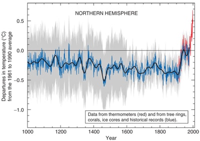
In the Holocene, the 11,200 year interval since the end of the last glacial period, the most obvious indicators of cool intervals in the past are moraines in mountainous areas, the stony mounds deposited by glaciers at various times in the past and situated at lower levels than present-day ice margins. Methods that have been used to date moraines include measuring the dimensions of the largest lichens growing on them, C14 dating of wood and other associated organic material and, more recently, Beryllium 10 dating of rock surfaces. It is necessary to attempt to differentiate the effects of precipitation and temperature on glacier advance and retreat (see Glossary). The results are inevitably imprecise as compared with daily measurements taken by a rain gauge or a thermometer in a Stevenson’s screen. Nevertheless, Oerlemans (2005) has shown that the record of advances and retreats of glacier fronts can provide temperature records that correspond closely with the instrumental record.
The annual layers of ice in cores extracted from ice caps in Greenland and Antarctica and sitting on the crests of high mountains in low latitudes have provided long records of climate change. Other means that have become available for attempting to discover past annual rainfall and temperature include making use of speleothems (stalagmites and stalactites –see Glossary–) in caves in limestone areas, dating the accretionary layers (see Glossary) by Uranium series age determinations, measuring the ∂18O isotope ratio (see Glossary) to obtain values for cave temperature, and measuring layer thicknesses as proxies for rainfall amounts. Extrapolating from the cave temperatures to conditions in the open air presents difficulties. Pollen cores from lakes or marshes provide a record of plant cover that can also give useful information about past temperatures, although there is a time lag between temperature change and vegetation change depending on the speed of plant migration and the distances that plant formations have had to cross.
Taken together, the record of climate change that has been obtained from these studies is coherent. An important feature is the evidence that climate changes in the past have commonly been abrupt, suggesting the possibility that build-up of greenhouse gases in the atmosphere could push the global climate system over a threshold, triggering an abrupt change to a new equilibrium.
The most dramatic sudden change in climate since the last glacial maximum was the sudden cooling about 12,800 years ago that brought cold, dry windy conditions to the North Atlantic region for 1,600 years during what is called the Younger Dryas. This event was caused by the climate warming and the sudden escape of enormous volumes of fresh water from under and around the decaying North American ice sheet, starting about 13,000 years ago and finding its way by the Mackenzie and other river valleys in north-west Canada to the Arctic Ocean (Murton et al., 2010). Reaching the North Atlantic the cold fresh water, being lighter than the warm salty water of the Gulf Stream, spread over the surface of the northernmost Atlantic bringing the Great Ocean Conveyor Belt (see Glossary) to a halt. The Ocean Conveyor[10] is the thermohaline circulation of the oceans. For several centuries before the Younger Dryas and for the last 10,000 years, it has allowed the Gulf Stream to reach northern latitudes. Off eastern Labrador and eastern Greenland the dense salty water brought north in the Gulf Stream has subsided to the depths of the Atlantic Ocean and made its way south, crossing the equator and rounding southern Africa to enter the Indian Ocean and even the Pacific Ocean before reaching up to the surface and returning to the North Atlantic by way of South Africa and the Gulf of Mexico (Broecker, 1989). With no North American ice sheet the situation today is quite different from that of 12,000 years ago, and the likelihood of the Ocean Conveyor ceasing to function is currently very slight.
Figure 19. Great Ocean Conveyor belt
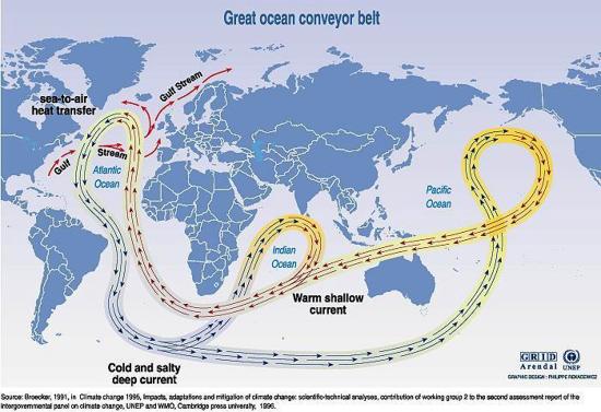
More relevant, as John Mercer warned 40 years ago, are the signs that the West Antarctic ice sheet may be unstable. The shelf-ice bordering the ice sheet has been breaking up and drifting away, allowing ice tongues to move seawards more rapidly. A group of 26 climate scientists issued a report in December 2009 which said that world sea-level rises had been about 80% higher than the IPCC had projected in 2001. If this process continues to accelerate it might allow the whole mass of ice to disintegrate and slide into the ocean, producing a rise in sea level of more than 3.3m.
Figure 20. West Antarctica, shown in red, has warmed far more than the east over the last 50 years
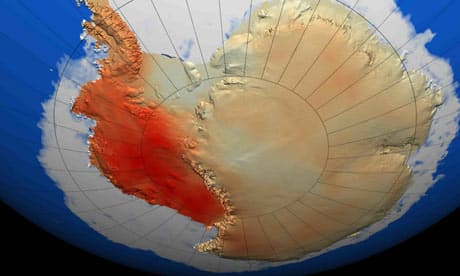
Figure 21. West Antarctica is a tightly coupled, dynamic environment
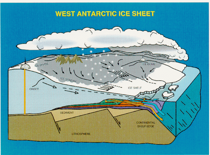
Source: R.A. Bindschadler et al., http://neptune.gsfc.nasa.gov/wais/articles/eos.html.
Annex 2. Glossary of Technical and Scientific Terms
Accretionary layers = Layerswhich make up stalagmites and stalactites located in caves in limestone areas.
Air bubbles in ice cores = Air bubbles trapped in ice, that are analysed by scientists extracting ice cores to be able to study variations in ancient climate. The accumulation of snow and ice over many years re-crystallises and in the process traps air bubbles from previous time periods. The composition of these ice cores, particularly the presence of hydrogen and oxygen isotopes provides an estimate of the climate at the time.
Albedo = The Earth’s reflectivity.
Black-body radiative disequilibrium = Thermal radiation from a black body is termed black-body radiation. In the blackbody spectrum, the shorter the wavelength, the higher the frequency, and higher frequency is related to higher temperature. Thus, the colour of a hotter object is closer to the blue end of the spectrum and the colour of a cooler object is closer to the red (from Wikipedia, http://en.wikipedia.org/wiki/Black_body).
BP (before present) = A time scale used in archaeology, geology and other scientific disciplines to specify when events in the past occurred. Because the ‘present’ time changes, standard practice is to use 1 January 1950 as the arbitrary origin of the age scale. For example, 1,500 BP means 1,500 years before 1950, that is, in the year 450 AD. BP can also be considered to be an abbreviation of Before Physics (http://en.wikipedia.org/wiki/Before_Present). The climate of a place is the sum total of its weather.
Cloud radiation processes = Cloud forcing (sometimes described as cloud radiative forcing) is the difference between the radiation budget components for average cloud conditions and cloud-free conditions. Much of the interest in cloud forcing relates to its role as a feedback process in the present period of global warming (from Wikipedia).
Cryosphere (glaciers and ice sheets) = Derived from the Greek word cryo for ‘cold’ or ‘to cool’. The term which collectively describes the portions of the Earth’s surface where water is in solid form, including sea ice, lake ice, river ice, snow cover, glaciers, ice caps and ice sheets, and frozen ground (which includes permafrost) (from Wikipedia).
Diatomite = The microscopic remains of algae that lived in an ancient lake, such as Mega Chad.
El Niño and La Niña = Names given to changes in the winds, atmospheric pressure and seawater that occur in the Pacific Ocean near the equator. El Niño and La Niña are opposite phases of a back and forth cycle in the Pacific Ocean and the atmosphere above it. Unlike winter and summer, however, El Niño and La Niña do not change with the regularity of the seasons; instead, they repeat on average about every three or four years. They are the extremes in a vast repeating cycle called the Southern Oscillation, El Niño being the warm extreme and La Niña the cold extreme (Lerner & Lerner, 2003).
EPICA Dome C = A European Project started in 1996 in Antarctica (EPICA) to drill an ice core from ice 3,270 metres thick at a site known as Dome C in East Antarctica. The aim was to provide the longest ice-core climate record yet, an archive of past environmental conditions on Earth and greenhouse gases over eight glacial cycles.
Great Ocean Conveyor Belt = An Ocean Conveyor is the thermohaline circulation of the oceans. For several centuries before the Younger Dryas and for the last 10,000 years it has allowed the Gulf Stream to reach northern latitudes.
Greenhouse gases (GHG) = The most abundant greenhouse gases are: water vapour, carbon dioxide, atmospheric methane, nitrous oxide, ozone and chlorofluorocarbons.
Harmattan = A dry and dusty West-African trade wind that blows south from the Sahara into the Gulf of Guinea between the end of November and the middle of March.
Indian Ocean Dipole (IOD) = An oceanographic phenomenon affecting climate in the Indian Ocean region The IOD involves an aperiodic oscillation of sea-surface temperatures, between ‘positive’, ‘neutral’ and ‘negative’ phases (from Wikipedia, http://en.wikipedia.org/wiki/Indian_Ocean_Dipole).
∂18O isotope ratio = Measuring the ∂18O isotope ratio to obtain values for cave temperature.
Lapse rate (including adiabatic lapse rate) = Defined as the rate of decrease with height for an atmospheric variable. The variable involved is temperature unless otherwise specified.
Large-scale overturning circulations = Atmospheric circulation is the large-scale movement of air, and the means (together with the smaller ocean circulation) by which thermal energy is distributed on the surface of the Earth (from Wikipedia, http://en.wikipedia.org/wiki/Atmospheric_circulation).
Last glacial maximum = The sudden cooling about 12,800 years ago that brought cold, dry windy conditions to the North-Atlantic region for 1,600 years during what is called the Younger Dryas glacier advance and retreat.
Little Ice Age = The record points to intervals within the last 700 years, each lasting several decades, when glaciers extended hundreds of metres further down their valleys than they do now. It has been called the Little Ice Age. The warming required to account for the retreat of Alpine glaciers from their most distant Little Ice Age moraines to their present positions is between 0.6º and 0.7oC, a value similar to that of global warming over the last 100 years.
Maunder Minimum = Also known as the prolonged sunspot minimum. The period roughly spanning 1645 to 1715 (as named by John A. Eddy in a landmark 1976 paper published in Science titled ‘The Maunder Minimum’) when sunspots became exceedingly rare as noted by solar observers of the time (from Wikipedia, http://en.wikipedia.org/wiki/Maunder_Minimum).
Moraines = Any glacially-formed accumulation of unconsolidated glacial debris (soil and rock) which can occur in currently glaciated and formerly glaciated regions, such as those areas acted upon by a past ice age.
Moulin = A narrow, tubular chute, hole or crevasse worn in the ice by surface water, which carries water from the surface to the base far below (from the French for ‘mill’). They can be up to 10 metres wide and are typically found at a flat area of a glacier in a region of transverse crevasses. These holes can go all the way to the bottom of the glacier and can be hundreds of metres deep, or may reach the depth of common crevasse formation (about 10-40 metres) where the stream flows englacially. These holes are a part of a glacier’s internal ‘plumbing’ system, to carry melt water out to wherever it may go. Water often exits the glacier at base level, but occasionally the lower end of a moulin may be exposed in the face of a glacier or at the edge of a stagnant block of ice (from http://www.global-greenhouse-warming.com/moulin.html).
Net forcing = The difference in climate directly attributed to current human activities.
Planktonic foraminifera = Dying planktonic foraminifera continuously rain down on the sea floor in vast numbers, their mineralised tests preserved as fossils in the accumulating sediment. Beginning in the 1960s, and largely under the auspices of the Deep Sea Drilling, Ocean Drilling andInternational Ocean Drilling Programmes, as well as for the purposes of oil exploration, advanced deep-sea drilling techniques have been bringing up sediment cores bearing foraminifera fossils by the millions. The effectively unlimited supply of these fossil tests and the relatively high-precision age-control models available for cores has produced an exceptionally high-quality planktonic foraminifera fossil record dating back to the mid-Jurassic, and presents an unparalleled record for scientists testing and documenting the evolutionary process. Calcareous fossil foraminifera are formed from elements found in the ancient seas they lived in. Thus they are very useful in paleoclimatology and paleoceanography. They can be used to reconstruct past climate by examining the stable isotope ratios of oxygen, and the history of the carbon cycle and oceanic productivity by examining the stable isotope ratios of carbon (from Wikipedia, http://en.wikipedia.org/wiki/Foraminifera).
Pollen cores from lakes or marshes = Pollen cores provide a record of plant cover and also useful information about past temperatures.
Precession (axial precession; precession of the equinoxes) = The Earth was nearer the sun during the Northern Hemisphere summer than it was to be later in the Holocene.
Speleothems = Stalagmites and stalactites located in caves in limestone areas, dating the accretionary layers.
Stomatal index = Leaves in a range of forest-tree species respond to rising concentrations of atmospheric COs over the last 200 years by a decrease in both osmatal density and stomatal index and therefore used as an indicator of Holocene atmospheric CO2 concentrations.
Threshold = The possibility that the build-up of greenhouse gases in the atmosphere could push the global climate system over a threshold, triggering an abrupt change to a new equilibrium.
Younger Dryas = An event was caused by climate warming and the sudden escape of enormous volumes of fresh water from under and around the decaying North-American ice sheet, starting about 13,000 years ago and finding its way by the Mackenzie and other river valleys in north-west Canada to the Arctic Ocean.
[1] Radiocarbon calibration: dates determined using radiocarbon dating come in two kinds: uncalibrated (also called Libby or raw) and calibrated (also called Cambridge) dates. Uncalibrated radiocarbon dates may be expressed using BP years; however, they are not identical to calendar dates. This has to do with the fact that the level of atmospheric radiocarbon (carbon-14 or 14C) has not been strictly constant during the span of time that can be radiocarbon-dated. Uncalibrated radiocarbon ages can be converted to calendar dates by means of calibration curves based on comparison of raw radiocarbon dates of samples independently dated by other methods, such as dendrochronology (dating on basis of tree growth-rings) and stratigraphy (dating on the basis of sediment layers in mud or sedimentary rock). Such calibrated dates are expressed as cal BP, where ‘cal’ indicates ‘calibrated years’ (extract from http://en.wikipedia.org/wiki/Before_Present).
[2] For more information see Jennifer McElwain & William G. Chaloner (1995), ‘Stomatal Density and Index of Fossil Plants Track Atmospheric Carbon Dioxide in the Palaeozoic’, Annals of Botany, nr 76, p. 389-395, http://aob.oxfordjournals.org/cgi/reprint/76/4/389.pdf.
[3] http://www.esrl.noaa.gov/gmd/ccgg/trends/#mlo_full.
[4] http://www.epa.gov/climatechange/emissions/co2_human.html.
[5] For an interactive explanation of albedo on Earth see http://www.windows2universe.org/earth/climate/sun_radiation_at_earth.html.
[6] http://eprints.lse.ac.uk/27939/1/HartwellPaper_English_version.pdf.
[7] Borehole records are a way of estimating the ground-surface temperature (GST) histories through borehole temperature profiles. For a brief explanation on glacial periods, see
http://www.acer-acre.org/ClimateChangeCD/sec4/421a.htm.
[8] Lerner & Lerner (2003).
[9] For detailed basic diagrams see http://www.windows2universe.org/earth/Atmosphere/earth_atmosph_radiation_budget.html.
[10] For a short paper on Great Ocean Conveyor see http://www.tos.org/oceanography/issues/issue_archive/issue_pdfs/4_2/4.2_broecker.pdf.
